Continuum mechanics/Functions

There are certain terms involving relationships between functions that you will often encounter in papers dealing with finite elements and continuum mechanics. We list some of the basic terms that you will see. More details can be found in books on advanced calculus and functional analysis.

Functions

Let $A$ and $B$ be two sets. A function is a rule that assigns to each $a \in A$ an element of $B$ . A function is usually denoted by

f : A \rightarrow B ~~~~(f~\text{takes}~A~\text{to}~B)~.

Sometimes, one also writes

a \mapsto f(a) ~~~~(a~\text{is mapped to the element}~f(a))~.

For example, if the function is $f(x) = x^2$ , then we may write $x \mapsto x^2$ .

Domain and Range

For a function $f : A \rightarrow B$ , the set $A$ is called the domain of $f$ . See Figure 1.

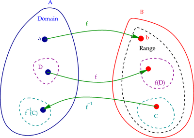Figure 1. Domain and range of a function.

The range of $f$ is the set

R(A) = \{ f(x) \in B ~|~ x \in A \}

Therefore, $R(A) \subset B$ .

One-to-one mapping (injection)

A function $f : A \rightarrow B$ is called one-to-one (or an injection) if no two distinct elements of $A$ are mapped to the same element of $B$ .

Onto mapping (surjection)

A function $f : A \rightarrow B$ is called onto if for every $b \in B$ there is an $a \in A$ such that $f(a) = b$ .

If that case, $R(A) = B$ .

One-to-one and onto mapping (bijection)

When a mapping is both one-to-one and onto it is called a bijection. For example, if $f : A \rightarrow B$ and $f(x) = x^2$ with

A = \{x \in \mathbb{R}^{} ~|~ x \ge 0\} ~;~~ B = \{x \in \mathbb{R}^{} ~|~ x \ge 0\}

the map is one-to-one and onto.

On the other hand if

A = \{x \in \mathbb{R}^{} ~|~ x \ge 0\} ~;~~ B = \{x \in \mathbb{R}^{}\}

the map is one-to-one but not onto.

If we choose

A = \{x \in \mathbb{R}^{}\} ~;~~ B = \{x \in \mathbb{R}^{}\}

the map is neither one-to-one nor onto.

Image, pre-image, and inverse functions

Suppose we have a function $f : A \rightarrow B$ . Let $D$ be a subset of $A$ (see Figure~1). Let us define

f(D) := \{f(d) \in B ~|~ d \in D\}~.

Then, $f(D)$ is called the image of $D$ .

On the other hand, if $C$ is a subset of $B$ and we define

f^{-1}(C) := \{a \in A ~|~ f(a) \in C\}~.

Then, $f^{-1}(C)$ is called the inverse image or pre-image of $C$ .

If $f : A \rightarrow B$ is one-to-one and onto, then there is a unique function $f^{-1} : B \rightarrow A$ such that

f(f^{-1}(b)) = b ~\text{for all}~ b\in B ~~~~~~\text{and}~~~~ f^{-1}(f(a)) = a ~\text{for all}~ a\in A ~.

The function $f^{-1}$ is called an inverse function of $f$ .

Identity map

The map $f : A \rightarrow A$ such that $f(x) = x$ for all $x \in A$ is called the identity map. This map is one-to-one and onto.

Composition

A notation that you will commonly see in papers on nonlinear solid mechanics is the composition of two functions. See Figure 2.

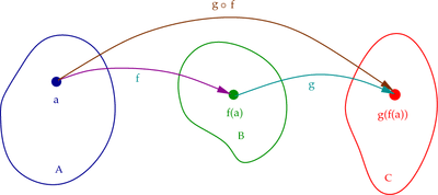Figure 2. Composition of functions.

Let $f$ and $g$ be two functions such that $f : A \rightarrow B$ and $g : B \rightarrow C$ . The composition $g \circ f : A \rightarrow C$ is defined as

g \circ f(a) := g(f(a))

Let us consider a stretch ( $f$ ) followed by a translation ( $g$ ). Then we can write $f : x \mapsto \lambda x$ and $g : y \mapsto y + c$ .

The composition $g \circ f$ is given by

g \circ f : x \mapsto \lambda x + c

The inverse composition $f \circ g$ is given by

f \circ g : x \mapsto \lambda(x + c)

Isomorphism and Homeomorphism

You will also come across the terms isomorphism and homeomorphism in the literature on nonlinear solid mechanics.

Isomorphism is a very general concept that appears in several areas of mathematics. The word means, roughly, "equal shapes". It usually refers to one-to-one and onto maps that preserve relations among elements.

A homeomorphism is a continuous transformation between two geometric figures that is continuous in both directions. The map has to be one-to-one to be homeomorphic. It also has to satisfy the requirements on an equivalence relation.

Continuously differentiable functions

A function

f : \Omega \rightarrow \mathbb{R}^{}

is said to be $k$ -times continuous differentiable or of class $C^k$ if its derivatives of order $j$ (where $0 \le j \le k$ ) exist and are continuous functions.

Figure 3 shows three functions ( $f(x)$ , $g(x)$ , $h(x)$ ) and their derivatives.

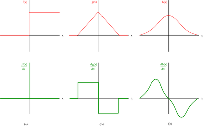Figure 3: Continuity of functions.

$C^{-1}$ Functions

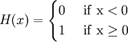
The function $f(x)$ is called the Heaviside step function (usually written $H(x)$ ) which is defined as

H(x) = \begin{cases} 0 & ~\rm{if}~ x < 0 \\ 1 & ~\rm{if}~ x \ge 0 \end{cases}

The derivative of the Heaviside function is the Dirac delta function (written $\delta(x)$ ) which has the defining property that

\int_{\infty}^{\infty} F(x)\delta(x-c)~dx = F(c)

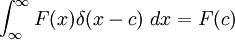
for any function $F(x)$ and any constant $c$ . The delta function is singular and discontinuous. Hence, the Heaviside function is not continuously differentiable. Sometimes the Heaviside function is said to belong to the class of $C^{-1}$ functions.

$C^0$ Functions

The function $g(x)$ in Figure 3 (also called a hat function) is continuous but has discontinuous derivatives. In this particular case, the function has the form

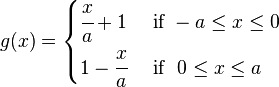
g(x) = \begin{cases} \cfrac{x}{a} +1 & ~\text{if}~ -a \le x \le 0 \\ 1 - \cfrac{x}{a} & ~\text{if}~~ 0 \le x \le a \end{cases}

Such functions that are differentiable only once are called $C^0$ functions.

$C^{\infty}$ Functions

The function $h(x)$ in Figure 3 is infinitely differentiable and has continuous derivatives every time it is differentiable. Such functions are called $C^{\infty}$ functions. Since the function can be differentiated once to give a continuous derivative, it also falls into the category of $C^1$ functions.

Sobolev spaces of functions

You will find Sobolev spaces being mentioned when you read the finite element literature. A clear understanding of these function spaces needs a knowledge of functional analysis. The book Introduction to Functional Analysis with Applications to Boundary Value Problems and Finite Elements by B. Daya Reddy is a good starting point that is just right for engineers. We will not get into the details here.

Of particular interest in finite element analysis are Sobolev spaces of functions such as

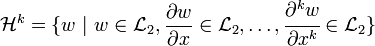
\mathcal{H}^k = \{w ~|~ w \in \mathcal{L}_2, \frac{\partial w}{\partial x} \in \mathcal{L}_2, \dots, \cfrac{\partial^k w}{\partial x^k} \in \mathcal{L}_2\}

where

\mathcal{L}_2 = \{w ~|~ \int_0^1 w^2 ~dx < \infty \} ~.

The function space $\mathcal{L}_2$ is the space of square integrable functions.

Of interest to us is an outcome of Sobolev's theorem which says that if a function is of class $\mathcal{H}^{k+1}$ then it is actually a bounded $C^k$ function. If we choose our basis functions from the set of square integrable functions with continuous derivatives, certain singularities are automatically precluded.

This article is issued from Wikiversity - version of the Thursday, August 16, 2007. The text is available under the Creative Commons Attribution/Share Alike but additional terms may apply for the media files.