Boundary Value Problems/Lesson 6

Return to BVP main page Boundary Value Problems

1D Wave Equation

Derivation of the wave equation using string model.

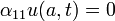
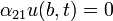
General form for boundary conditions.

$\alpha_{11} u(a,t) + \alpha_{12} u_x (a,t) = \gamma_{1}$ $\alpha_{21} u(b,t) + \alpha_{22} u_x (b,t) = \gamma_{2}$

Wave equation with Dirichlet Homogeneous Boundary conditions.

$\displaystyle \alpha_{11} u(a,t) = 0$
$\displaystyle \alpha_{21} u(b,t) = 0$
In the homogeneous problem 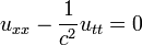$\displaystyle u_{xx}-\frac{1}{c^2} u_{tt} =0$ with $\displaystyle u(0,t) =0$ , $\displaystyle u(L,t) =0$

Finding a solution: u(x,t)

Let 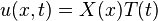$u(x,t)= X(x)T(t)$
then substitute this into the PDE.
$X'' T = \frac{1}{c^2} X T''$
$\frac{X''}{X} = \frac{1}{c^2} \frac{T''}{T} = \mu$
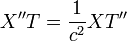
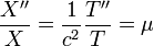
Where $\mu$ is a constant that can be positive, zero or negative. We need to check each case for a solution.

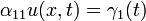
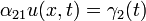
Wave Equation with nonhomogeneous Dirichlet Boundary Conditions

In the homogeneous problem $u_{xx}-\frac{1}{c^2} u_{tt} =0$
$\displaystyle \alpha_{11} u(x,t) = \gamma_{1}(t)$
$\displaystyle \alpha_{21} u(x,t) = \gamma_{2} (t)$

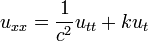
Wave Equation with resistive damping

In the homogeneous problem $u_{xx}=\frac{1}{c^2} u_{tt} + ku_t$

This article is issued from Wikiversity - version of the Saturday, August 30, 2014. The text is available under the Creative Commons Attribution/Share Alike but additional terms may apply for the media files.