Boundary Value Problems/Lesson 5.2

Click here to return to BVPs Boundary Value Problems

Title: One 1D heat equation with several boundary conditions
Objectives: Specifically what is to be retained by the learner.
1. Setup of heat equation
2. Solution of heat equation with homogeneous/nonhomogeneous Dirichlet, Neumann and mixed boudary conditions.
Activities: Content directed at the learner to achieve learning objectives.
1. Solve specific homework prooblems.
Assessment: Determine lesson effectiveness in achieving the learning Objectives.
1. Homework and quizzes

Background

The derivation of the Heat Equation

Heat Flow: Fourier's Law

What is heat? Heat is a form of energy that is measured in units of degree Celsius ^[1].

For a gas this measure is the average kinetic energy 
  $m |v|^2 / 2$  of the molecules in the gas.

For a solid heat is associated with vibrational energy of the crystalline structure.
Heat is measured by us in units of degrees, these are related to calories by the definition, one calorie is the amount of heat required to increase the temperature of one gram of water(at one atmosphere of pressure) by one degree Celsius.

References

↑ a historical form of energy measurement is the calorie which is the amount of heat required to increase the temperature of one gram of water(at one atmosphere of pressure) by one degree Celsius.

How heat flows?

Let $\Omega$ represent a region of space in $\mathbf{R}^3$ and $u(x,y,z,t)$ be the temperature at a point in $\Omega$ at a time $t$ . From observation you know that heat flows from a high temperature region to a lower temperature region. Mathematically we represent this as $- \nabla u$ which is a vector pointing in the direction of decreasing temperatures. The negative gradient of $u$ is a vector that points in the direction that the temperature is decreasing the most. Heat is flowing in that direction, at least locally.

The heat flux vector $v = -\nabla u$ describes a vector field in $\Omega$ for the scalar field $u(x,y,z,t)$ .

Think of $S$ as a a surface in $\Omega$ . As shown below.
Fourier's Law
$\mbox{heat flux across S in the direction normal to the surface S} = - \kappa (\nabla{u} \cdot n)A$

Insulated Rod with ends held at fixed temperatures.

The temperature in a bar extending from $x=a$ to $x=b$ at a time $t$ is $u(x,t)$ . The flow of heat in the bar leads to the development of the General Heat Equation in one spatial dimension. At this time I have not entered the material for this from my notes. It is found in a variety of standard BVP and DE textbooks. The derivation leads to the following PDE with boundary conditions and initial condition.
The general form for the heat equation in one spatial dimension is:

PDE 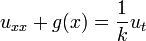$u_{xx}+ g(x) = \frac {1}{k} u_t$ with the general boundary conditions
$\displaystyle \alpha_{11} u(a,t) + \alpha_{12} u_x(a,t) = \gamma_1(t)$
$\displaystyle \alpha_{21} u(b,t) + \alpha_{22} u_x(b,t) = \gamma_2(t)$
and the initial condition 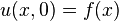$u(x,0)=f(x)$ for $a \leq x \leq b$ .

Dirichlet Boundary Conditions: If $\alpha_{12}=\alpha_{22}=0$ the problem is said to have Dirichlet boundary conditions.

$\displaystyle u(0,t)=3,u(L,t)=10$ where $a=0,b=L$ are Dirichlet BCs. For this introductory work $g(x)=0$ and $\gamma_1(t),\gamma_2(t)$ are constants.
This will give us the simpler problem $\displaystyle u_{xx} =\frac {1}{k} u_t$ with the boundary conditions
$\displaystyle \alpha_{11} u(a,t) + \alpha_{12} u_x(a,t) = \gamma_1 =constant$
$\displaystyle \alpha_{21} u(b,t) + \alpha_{22} u_x(b,t) = \gamma_2 =constant$
and the initial condition $\displaystyle u(x,0)=f(x)$ for $\displaystyle a \leq x \leq b$ .

We first solve the problem with the BCs set to a fixed temperature of $\displaystyle u(a,t)=0 ,u(b,t)=0$ . The case is the result of setting $\displaystyle \alpha_{11}=\alpha{21}=1,\alpha_{21}=\alpha{22}=0$ and $\displaystyle \gamma_1=\gamma_2=0$

Homogeneous Boundary conditions for fixed end temperatures, Dirichlet

The rod is insulated along it's length and contains no sources or sinks is $\displaystyle g(x)=0$ :

$\displaystyle u_{xx}=\frac {1}{k} u_t$

Insulated Rod with ends held at fixed temperatures.

The general form for the accompanying boundary conditions at either end of the rod is:

$\displaystyle u(a,t) =0 \mbox { and } u(b,t)=0$ . Setting $a=0 , b=L$ we have $u(0,t) =0, u(L,t)=0$ .

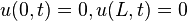A quick knowledge check:

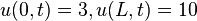
Lesson on Heat equation in 1D with Nonhomogeneous Dirichlet Boundary Conditions

Solve a nonhomogeneous Dirichlet BC problems.

  $\displaystyle \gamma_1(a,t) \neq 0,\gamma_2(b,t)\neq 0$  and  $\alpha_{12} = \alpha_{22}=0$ .

Setup the PDE and BCs

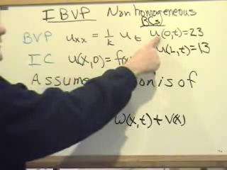
Suppose the solution consists of a transitory component $w(x,t)$ and a steady state component $v(x)$ . To solve for $u(x,t)$ we will develop two problems. One will be assigned the nonhomogeneous BCs, $v_{xx}=0$ with nonzero end conditions $v(a),v(b)$ and the second problem will be assigned homogeneous BCs and the IC, $w_{xx}= \frac{1}{k} w_t$ with zero end conditions 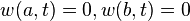$w(a,t)=0,w(b,t)=0$ and $w(x,0)=f(x)-v(x)$ .

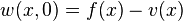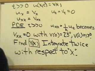
Solve for steady state part of the solution $v(x)$

Video OK click on play. Setup for steady state v(x) part of the solution.

Just CLICK on the play button and the video will work , currently the thumnails for the uploads are messed up.

Video OK Click on play.

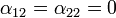
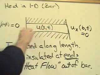
Neumann

The Neumann end condition is a first derivative condition on the heat flow across an end of the bar. The homogeneous case would have no heat flow, across a boundary

$\displaystyle \alpha_{11} = \alpha_{21} = 0$ and $\alpha_{12} \neq 0 , \alpha_{22} \neq 0$ for all "t" and so

$u_x(a,t)=0$ and $u_x(b,t)=0$ at the left and right boundaries when $\gamma_1(t) = \gamma_2(t)=0$ .

Insulated Rod with Homogeneous Neumann

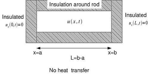
These are conditions where no heat flows across the ends of the rod. Thus no energy may enter or leave the rod.

Solution

Click on the PLAY arrow, video works. The thumbnails' jpeg images are the only thing messed up.

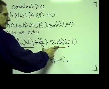
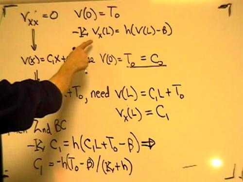
Mixed: Fixed Temp and Convection

$\displaystyle u_{xx} =\frac {1}{k} u_t$ with the boundary conditions
$\displaystyle u(0,t)= T_0$ and $\displaystyle -\kappa u_x(b,t) = h(u(L,t)- \Beta)$
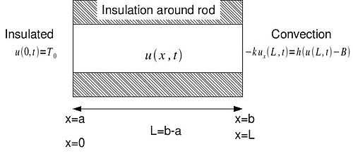
and the initial condition $\displaystyle u(x,0)=f(x)$ for $\displaystyle a \leq x \leq b$ .

Heat Equation 1D mixed boundary conditions.

Lecture on setup of Heat equation for an insulated bar with one end held at a fixed temperature and the convective cooling applied to the second.

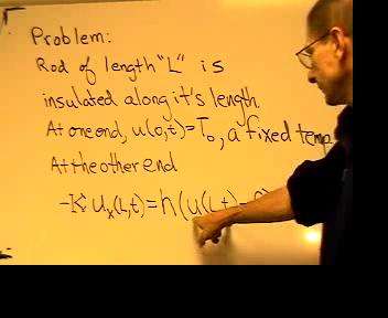
Lecture on solving for the steady steady $v(x)$ of Heat equation for an insulated bar with one end held at a fixed temperature and the convective cooling applied to the second.

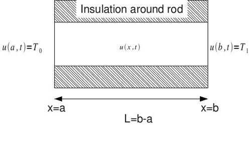
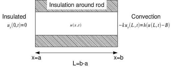
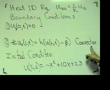
Heat 1d : Insulated and convective BCs

A bar of length L is insulated along it's length. One end is open to the air which is at $\Beta$ degrees and the other end is insulated so that there is no flow across the boundary.
The heat equation is then: $\displaystyle u_{xx} =\frac {1}{k} u_t$ with the boundary condition s
$u_x(0,t)=0$ at the insulated end and $-\kappa u_x(L,t) = h ( u(L,t)- \Beta)$ at the convective end.

Heat Equation 1D mixed boundary conditions: insulated and convective BCs.

The intial temperature distribution is given by the function: $u(x,0)=f(x)=-x^2+10x+23$
Just click on the Play button and video works!. The first video sets up the problem and starts the solution process.

The next video continues with the solution of the transient part of the problem.

This last video completes the transient solution and writes the series solution u(x,t).

This article is issued from Wikiversity - version of the Saturday, August 30, 2014. The text is available under the Creative Commons Attribution/Share Alike but additional terms may apply for the media files.

	$\displaystyle u(a,t)=20$
	$\displaystyle u_x(0,t)=0$
	$\displaystyle u(L,t)=u_x(L,t)$