B Splines

Please see Directions for use for more information.

Learning Project Summary

Portals: Learning Projects, Engineering and Technology
School: Computer Science
Department: Scientific Computing

Content summary

This learning project aims to provide as an introduction to the specialized spline functions known as B (or Basis) splines. B splines have varying applications, including numerical analysis.

Goals

Define B Spline
Differentiate types of B Splines
Approximation using B Splines

Lessons

Lesson 0: Prerequisite

B splines derive from Splines, therefore an understanding of Splines in general is beneficial to completing this lesson. In short, a Spline function approximates another function by defining a set of polynomials

$S_0(x),\ S_1(x), \ldots,S_n(x)$

where each of these polynomials defines a specific piece of the resulting Spline. $S_0(x)$ might exist on the interval $[0,1]$ , $S_1(x)$ might exist on the interval $[1,2]$ , and so on. The result will be a piecewise approximation to some other exact function.

Lesson 1: Definition

A definition of B splines assumes:

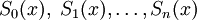
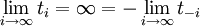
an infinite set of knots are defined at points along the x-axis (can be spaced uniformally or not), that is,
- $\ldots < t_{-2} < t_{-1} < t_0 < t_1 < t_2\ \ldots$
- $\lim_{i\rightarrow \infty} t_{i} = \infty = -\lim_{i\rightarrow \infty} t_{-i}$

Degree 0 (or constant)

With that in mind, we can now move on to the simplest of B splines, those of degree 0, which are defined as

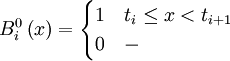
$B_i^0\left ( x \right ) = \begin{cases}1 & t_{i} \le x < t_{i+1}\\0 & -\end{cases}$

In other words, a degree 0 B spline is equal to 0 at all points except on the interval $\left [ t_{i},t_{i+1} \right )$ .

It should now be easy to see that a degree 0 Spline can be formed as a weighted linear combination of degree 0 B splines so that,

$S = \ldots + b_{i-1}B_{i-1}^0 + b_{i}B_{i}^0 + b_{i+1}B_{i+1}^0 + \ldots$
$-\infty <= i <= \infty$

Degree 1 (or linear)

Logically, the next B spline are those of degree 1, defined as

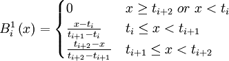
$B_i^1\left ( x \right ) = \begin{cases}0 & x \ge t_{i+2}\ or\ x < t_{i}\\\frac{x - t_{i}}{t_{i+1} - t_{i}} & t_{i} \le x < t_{i+1}\\\frac{t_{i+2} - x}{t_{i+2} - t_{i+1}} & t_{i+1} \le x < t_{i+2}\end{cases}$

This might seem difficult to visualize at first glance, but its actually quite easy. Just like $B_{i}^0$ , it is 0 at quite nearly all points. However, we now have the two intervals, $\left [ t_{i},t_{i+1} \right )$ and $\left [ t_{i+1},t_{i+2} \right )$ , at which $B_{i}^1 \ne 0$ .

On the first interval it is easy to see that, substituting $t_{i}$ and $t_{i+1}$ give 0 and 1, respectively. Thus, this function yields an upward sloping line, with a maximum height of 1. Similarly, the second interval yields a downward sloping line, starting from the point that the first interval terminates.

Again, similarly to $B_{i}^0$ , it should now be easy to see that a degree 1 Spline can be formed as a weighted linear combination of degree 1 B splines so that,

$S = \ldots + b_{i-1}B_{i-1}^1 + b_{i}B_{i}^1 + b_{i+1}B_{i+1}^1 + \ldots$
$-\infty <= i <= \infty$

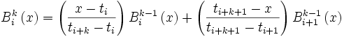
Degree k (or quadratic and above)

The higher degree B splines, and actually including $B_{i}^1$ , are defined as

$B_{i}^k\left ( x \right ) = \left ( \frac{x - t_{i}}{t_{i+k} - t_{i}} \right ) B_{i}^{k-1}\left ( x \right ) + \left ( \frac{t_{i+k+1} - x}{t_{i+k+1} - t_{i+1}} \right ) B_{i+1}^{k-1}\left ( x \right )$

Lesson 2: Approximation

We have seen how B splines can be used to construct general Spline. Now we will discuss a process for approximating a generic function by using B splines.

Schoenberg's Approximation

This specific approximation utilizes $B_{i}^2$ (or quadratic B splines) to approximate a function with $S^2$ (or a quadratic Spline). The approximation is defined as

$S \left ( x \right ) = \ldots + f \left ( \tau_{i-1} \right ) B_{i-1}^2 + f \left ( \tau_{i} \right ) B_{i}^2 + f \left ( \tau_{i+1} \right ) B_{i+1}^2 + \ldots$
$-\infty <= i <= \infty$
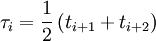$\tau_{i} = \frac{1}{2} \left ( t_{i+1} + t_{i+2} \right )$ , or the average of the next two knots

In real life, we would only approximate the function over a specific interval $\left [ a,b \right ]$ .

References

Additional helpful readings include:

<---include subject name

Active participants

Active participants in this Learning Group

Jlietz 18:04, 12 December 2006 (UTC)

This article is issued from Wikiversity - version of the Sunday, June 17, 2012. The text is available under the Creative Commons Attribution/Share Alike but additional terms may apply for the media files.