Applied linear operators and spectral methods/Lecture 4

< Applied linear operators and spectral methods

More on spectral decompositions

In the course of the previous lecture we essentially proved the following theorem:

Theorem:

1) If a $n\times n$ matrix $\mathbf{A}$ has $n$ linearly independent real or complex eigenvectors, the $\mathbf{A}$ can be diagonalized. 2) If $\mathbf{T}$ is a matrix whose columns are eigenvectors then $\mathbf{T}\mathbf{A}\mathbf{T}^{-1}= \boldsymbol{\Lambda}$ is the diagonal matrix of eigenvalues.

The factorization $\mathbf{A} = \mathbf{T}^{-1}\boldsymbol{\Lambda}\mathbf{T}$ is called the spectral representation of $\mathbf{A}$ .

Application

We can use the spectral representation to solve a system of linear homogeneous ordinary differential equations.

For example, we could wish to solve the system

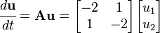
\cfrac{d\mathbf{u}}{dt} = \mathbf{A}\mathbf{u} = \begin{bmatrix}-2 & 1 \\ 1 & -2 \end{bmatrix} \begin{bmatrix} u_1 \\ u_2 \end{bmatrix}

(More generally $\mathbf{A}$ could be a $n \times n$ matrix.)

Comment:

Higher order ordinary differential equations can be reduced to this form. For example,

\cfrac{d^2u_1}{dt^2} + a~\cfrac{du_1}{dt} = b~u_1

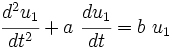
Introduce

u_2 = \cfrac{du_1}{dt}

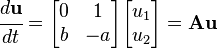
Then the system of equations is

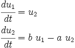
\begin{align} \cfrac{du_1}{dt} & = u_2 \\ \cfrac{du_2}{dt} & = b~u_1 - a~u_2 \end{align}

or,

\cfrac{d\mathbf{u}}{dt} = \begin{bmatrix} 0 & 1 \\ b & -a \end{bmatrix} \begin{bmatrix} u_1 \\ u_2 \end{bmatrix} = \mathbf{A} \mathbf{u}

Returning to the original problem, let us find the eigenvalues and eigenvectors of $\mathbf{A}$ . The characteristic equation is

det(\mathbf{A} - \lambda~\mathbf{I}) = 0

o we can calculate the eigenvalues as

(2+\lambda)(2+\lambda) - 1 = 0 \quad \implies \quad \lambda^2 + 4\lambda + 3 = 0 \qquad \implies \qquad \lambda_1 = -1, \qquad \lambda_2= -3

The eigenvectors are given by

(\mathbf{A} - \lambda_1~\mathbf{I})\mathbf{n}_1 = \mathbf{0} ~;~~ (\mathbf{A} - \lambda_2~\mathbf{I})\mathbf{n}_2 = \mathbf{0}

or,

-n_1^1 + n_2^1 = 0 ~;~~ n_1^1 - n_2^1 = 0 ~;~~ n_1^2 + n_2^2 = 0 ~;~~ n_1^2 + n_2^2 = 0

Possible choices of $\mathbf{n}_1$ and $\mathbf{n}_2$ are

\mathbf{n}_1 = \begin{bmatrix} 1 \\ 1 \end{bmatrix} ~;~~ \mathbf{n}_2 = \begin{bmatrix} 1 \\ -1 \end{bmatrix}

The matrix $\mathbf{T}$ is one whose columd are the eigenvectors of $\mathbf{A}$ , i.e.,

\mathbf{T} = \begin{bmatrix} 1 & 1 \\ 1 & -1 \end{bmatrix}

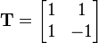
and

\boldsymbol{\Lambda} = \mathbf{T}^{-1} \mathbf{A} \mathbf{T} = \begin{bmatrix} -1 & 0 \\ 0 & -3 \end{bmatrix}

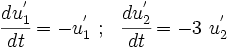
If $\mathbf{u} = \mathbf{T} \mathbf{u}^{'}$ the system of equations becomes

\cfrac{d\mathbf{u}^{'}}{dt} = \mathbf{T}^{-1} \mathbf{A} \mathbf{T} \mathbf{u}^{'} = \boldsymbol{\Lambda}~\mathbf{u}^{'}

Expanded out

\cfrac{du_1^{'}}{dt} = - u_1^{'} ~;~~ \cfrac{du_2^{'}}{dt} = - 3~u_2^{'}

The solutions of these equations are

u_1^{'} = C_1~e^{-t} ~;~~ u_2^{'} = C_2~e^{-3t}

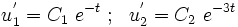
Therefore,

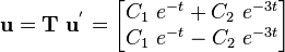
\mathbf{u} = \mathbf{T}~\mathbf{u}^{'} = \begin{bmatrix} C_1~e^{-t} + C_2~e^{-3t} \\ C_1~e^{-t} - C_2~e^{-3t} \end{bmatrix}

This is the solution of the system of ODEs that we seek.

Most "generic" matrices have linearly independent eigenvectors. Generally a matrix will have $n$ distinct eigenvalues unless there are symmetries that lead to repeated values.

Theorem

If $\mathbf{A}$ has $k$ distinct eigenvalues then it has $k$ linearly independent eigenvectors.

Proof:

We prove this by induction.

Let $\mathbf{n}_j$ be the eigenvector corresponding to the eigenvalue $\lambda_j$ . Suppose $\mathbf{n}_1, \mathbf{n}_2, \dots, \mathbf{n}_{k-1}$ are linearly independent (note that this is true for $k$ = 2). The question then becomes: Do there exist $\alpha_1, \alpha_2, \dots, \alpha_k$ not all zero such that the linear combination

\alpha_1~\mathbf{n}_1 + \alpha_2~\mathbf{n}_2 + \dots + \alpha_k~\mathbf{n}_k = 0

Let us multiply the above by $(\mathbf{A} - \lambda_k~\mathbf{I})$ . Then, since $\mathbf{A}~\mathbf{n}_i = \lambda_i~\mathbf{n}_i$ , we have

\alpha_1~(\lambda_1 - \lambda_k)~\mathbf{n}_1 + \alpha_2~(\lambda_2 - \lambda_k)~\mathbf{n}_2 + \dots + \alpha_{k-1}~(\lambda_{k-1} - \lambda_k)~\mathbf{n}_{k-1} + \alpha_k~(\lambda_k - \lambda_k)~\mathbf{n}_k = \mathbf{0}

Since $\lambda_k$ is arbitrary, the above is true only when

\alpha_1 = \alpha_2 = \dots = \alpha_{k-1} = 0

In thast case we must have

\alpha_k~\mathbf{n}_k = \mathbf{0} \quad \implies \quad \alpha_k = 0

This leads to a contradiction.

Therefore $\mathbf{n}_1, \mathbf{n}_2, \dots, \mathbf{n}_k$ are linearly independent. $\qquad \square$

Another important class of matrices which are diagonalizable are those which are self-adjoint.

Theorem

If $\boldsymbol{A}$ is self-adjoint the following statements are true

$\langle \boldsymbol{A}\mathbf{x}, \mathbf{x} \rangle$ is real for all $\mathbf{x}$ .
All eigenvalues are real.
Eigenvectors of distinct eigenvalues are orthogonal.
There is an orthonormal basis formed by the eigenvectors.
The matrix $\boldsymbol{A}$ can be diagonalized (this is a consequence of the previous statement.)

Proof

1) Because the matrix is self-adjoint we have

\langle \boldsymbol{A}\mathbf{x}, \mathbf{x} \rangle = \langle \mathbf{x}, \boldsymbol{A}\mathbf{x} \rangle

From the property of the inner product we have

\langle \mathbf{x}, \boldsymbol{A}\mathbf{x} \rangle = \overline{\langle \boldsymbol{A}\mathbf{x}, \mathbf{x} \rangle}

Therefore,

\langle \boldsymbol{A}\mathbf{x}, \mathbf{x} \rangle = \overline{\langle \boldsymbol{A}\mathbf{x}, \mathbf{x} \rangle}

which implies that $\langle \boldsymbol{A}\mathbf{x}, \mathbf{x} \rangle$ is real.

2) Since $\langle \boldsymbol{A}\mathbf{x}, \mathbf{x} \rangle$ is real, $\langle \boldsymbol{I}\mathbf{x}, \mathbf{x} \rangle = \langle \mathbf{x},\mathbf{x} \rangle$ is real. Also, from the eiegnevalue problem, we have

\langle \boldsymbol{A}\mathbf{x}, \mathbf{x} \rangle = \lambda~\langle \mathbf{x}, \mathbf{x} \rangle

Therefore, $\lambda$ is real.

3) If $(\lambda,\mathbf{x})$ and $(\mu, \mathbf{y})$ are two eigenpairs then

\lambda~\langle \mathbf{x}, \mathbf{y} \rangle = \langle \boldsymbol{A}\mathbf{x}, \mathbf{y} \rangle

Since the matrix is self-adjoint, we have

\lambda~\langle \mathbf{x}, \mathbf{y} \rangle = \langle \mathbf{x}, \boldsymbol{A}\mathbf{y} \rangle = \mu~\langle \mathbf{x}, \mathbf{y} \rangle

Therefore, if $\lambda \ne \mu \ne 0$ , we must have

\langle \mathbf{x}, \mathbf{y} \rangle = 0

Hence the eigenvectors are orthogonal.

4) This part is a bit more involved. We need to define a manifold first.

Linear manifold

A linear manifold (or vector subspace) $\mathcal{M} \in \mathcal{S}$ is a subset of $\mathcal{S}$ which is closed under scalar multiplication and vector addition.

Examples are a line through the origin of $n$ -dimensional space, a plane through the origin, the whole space, the zero vector, etc.

Invariant manifold

An invariant manifold $\mathcal{M}$ for the matrix $\boldsymbol{A}$ is the linear manifold for which $\mathbf{x} \in \mathcal{M}$ implies $\boldsymbol{A}\mathbf{x} \in \mathcal{M}$ .

Examples are the null space and range of a matrix $\boldsymbol{A}$ . For the case of a rotation about an axis through the origin in $n$ -space, invaraiant manifolds are the origin, the plane perpendicular to the axis, the whole space, and the axis itself.

Therefore, if $\mathbf{x}_1, \mathbf{x}_2, \dots,\mathbf{x}_m$ are a basis for $\mathcal{M}$ and $\mathbf{x}_{m+1}, \dots, \mathbf{x}_n$ are a basis for $\mathcal{M}_\perp$ (the perpendicular component of $\mathcal{M}$ ) then in this basis $\boldsymbol{A}$ has the representation

\boldsymbol{A} = \begin{bmatrix} x & x & | & x & x \\ x & x & | & x & x \\ - & - & - & - & - \\ 0 & 0 & | & x & x \\ 0 & 0 & | & x & x \end{bmatrix}

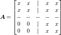
We need a matrix of this form for it to be in an invariant manifold for $\boldsymbol{A}$ .

Note that if $\mathcal{M}$ is an invariant manifold of $\boldsymbol{A}$ it does not follow that $\mathcal{M}_\perp$ is also an invariant manifold.

Now, if $\boldsymbol{A}$ is self adjoint then the entries in the off-diagonal spots must be zero too. In that case, $\boldsymbol{A}$ is block diagonal in this basis.

Getting back to part (4), we know that there exists at least one eigenpair ( $\lambda_1, \mathbf{x}_1$ ) (this is true for any matrix). We now use induction. Suppose that we have found ( $n-1$ ) mutually orthogonal eigenvectors $\mathbf{x}_i$ with $\boldsymbol{A}\mathbf{x}_i = \lambda_i\mathbf{x}_i$ and $\lambda_i$ are real, $i = 1, \dots, k-1$ . Note that the $\mathbf{x}_i$ s are invariant manifolds of $\boldsymbol{A}$ as is the space spanned by the $\mathbf{x}_i$ s and so is the manifold perpendicular to these vectors).

We form the linear manifold

\mathcal{M}_k = \{\mathbf{x} | \langle \mathbf{x}, \mathbf{x}_j \rangle = 0 ~~ j = 1, 2, \dots, k-1\}

This is the orthogonal component of the $k-1$ eigenvectors $\mathbf{x}_1, \mathbf{x}_2, \dots, \mathbf{x}_{k-1}$ If $\mathbf{x} \in \mathcal{M}_k$ then

\langle \mathbf{x}, \mathbf{x}_j \rangle = 0 \quad \text{and} \quad \langle \boldsymbol{A}\mathbf{x}, \mathbf{x}_j \rangle = \langle \mathbf{x}, \boldsymbol{A}\mathbf{x}_j \rangle = \lambda_j\langle \mathbf{x}, \mathbf{x}_j \rangle = 0

Therefore $\boldsymbol{A}\mathbf{x} \in \mathcal{M}_k$ which means that $\mathcal{M}_k$ is invariant.

Hence $\mathcal{M}_k$ contains at least one eigenvector $\mathbf{x}_k$ with real eigenvalue $\lambda_k$ . We can repeat the procedure to get a diagonal matrix in the lower block of the block diagonal representation of $\boldsymbol{A}$ . We then get $n$ distinct eigenvectors and so $\boldsymbol{A}$ can be diagonalized. This implies that the eigenvectors form an orthonormal basis.

5) This follows from the previous result because each eigenvector can be normalized so that $\langle \mathbf{x}_i, \mathbf{x}_j \rangle = \delta_{ij}$ .

We will explore some more of these ideas in the next lecture.

Resource type: this resource contains a lecture or lecture notes.

Action required: please create Category:Applied linear operators and spectral methods/Lectures and add it to Category:Lectures.

This article is issued from Wikiversity - version of the Monday, September 13, 2010. The text is available under the Creative Commons Attribution/Share Alike but additional terms may apply for the media files.