Applied linear operators and spectral methods/Lecture 3

< Applied linear operators and spectral methods

Review

In the last lecture we talked about norms in inner product spaces. The induced norm was defined as

\lVert\mathbf{x}\rVert = \sqrt{\langle \mathbf{x}, \mathbf{x} \rangle} = \lVert\mathbf{x}\rVert_2 ~.

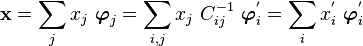
We also talked about orthonomal bases and biorthonormal bases. The biorthonormal bases may be thought of as dual bases in the sense that covariant and contravariant vector bases are dual.

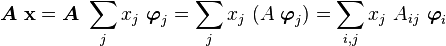
The last thing we talked about was the idea of a linear operator. Recall that

\boldsymbol{A}~\boldsymbol{\varphi}_j = \sum_i A_{ij}~\varphi_i \equiv A_{ij}~\varphi_i

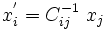
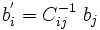
where the summation is on the first index.

In this lecture we will learn about adjoint operators, Jacobi tridiagonalization, and a bit about the spectral theory of matrices.

Adjoint operator

Assume that we have a vector space with an orthonormal basis. Then

\langle \boldsymbol{A}~\boldsymbol{\varphi}_j, \boldsymbol{\varphi}_i \rangle = A_{kj}~\langle \boldsymbol{\varphi}_k, \boldsymbol{\varphi}_i \rangle = A_{kj}~\delta_{ki} = A_{ij}

One specific matrix connected with $\boldsymbol{A}$ is the Hermitian conjugate matrix. This matrix is defined as

A_{ij}^{*} = \overline{A}_{ji}

The linear operator $\boldsymbol{A}^{*}$ connected with the Hermitian matrix is called the adjoint operator and is defined as

\boldsymbol{A}^* = \overline{\boldsymbol{A}}^T

Therefore,

\langle \boldsymbol{A}^{*}~\boldsymbol{\varphi}_j, \boldsymbol{\varphi}_i \rangle = \overline{A}_{ji}

and

\langle \boldsymbol{\varphi}_i, \boldsymbol{A}^{*}~\boldsymbol{\varphi}_j \rangle = A_{ji} = \langle \boldsymbol{A}~\boldsymbol{\varphi}_i, \boldsymbol{\varphi}_j \rangle

More generally, if

\mathbf{f} = \sum_i \alpha_i~\boldsymbol{\varphi}_i \qquad \text{and} \qquad \mathbf{g} = \sum_j \beta_j~\boldsymbol{\varphi}_j

then

\langle \mathbf{f}, \boldsymbol{A}^{*} ~\mathbf{g}\rangle = \sum_{i,j} \alpha_i~\overline{\beta}_j \langle \boldsymbol{\varphi}_i, \boldsymbol{A}^{*} ~\boldsymbol{\varphi}_j\rangle = \sum_{i,j} \alpha_i~\overline{\beta}_j \langle \boldsymbol{A}~\boldsymbol{\varphi}_i, \boldsymbol{\varphi}_j \rangle = \langle \boldsymbol{A}~\mathbf{f}, \mathbf{g} \rangle

Since the above relation does not involve the basis we see that the adjoint operator is also basis independent.

Self-adjoint/Hermitian matrices

If $\boldsymbol{A}^{*} = \boldsymbol{A}$ we say that $\boldsymbol{A}$ is self-adjoint, i.e., $A_{ij} = \overline{A}_{ji}$ in any orthonomal basis, and the matrix $A_{ij}$ is said to be Hermitian.

Anti-Hermitian matrices

A matrix $\mathbf{B}$ is anti-Hermitian if

B_{ij} = - \overline{B}_{ji}

There is a close connection between Hermitian and anti-Hermitian matrices. Consider a matrix $\mathbf{A} = i~\mathbf{B}$ . Then

A_{ij} = i~B_{ij} = -i~\overline{B}_{ji} = \overline{A}_{ji} ~.

Jacobi Tridiagonalization

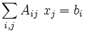
Let $\boldsymbol{A}$ be self-adjoint and suppose that we want to solve

(\boldsymbol{I} - \lambda~\boldsymbol{A})~\mathbf{y} =\mathbf{b}

where $\lambda$ is constant. We expect that

\mathbf{y} = (\boldsymbol{I} - \lambda~\boldsymbol{A})^{-1}~\mathbf{b}

If $\lambda~\mathbf{a}$ is "sufficiently" small, then

\mathbf{y} = (\boldsymbol{I} + \lambda~\boldsymbol{A} + \lambda^2~\boldsymbol{A}^2 + \lambda^3~\boldsymbol{A}^3 + \dots)~\mathbf{b}

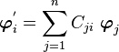
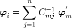
This suggest that the solution should be in the subspace spanned by $\mathbf{b}, \boldsymbol{A}~\mathbf{b}, \boldsymbol{A}^2~\mathbf{b}, \dots$ .

Let us apply the Gram-Schmidt orthogonalization procedure where

\mathbf{x}_1 = \mathbf{b},~ \mathbf{x}_2 = \boldsymbol{A}~\mathbf{b}, ~ \mathbf{x}_3 = \boldsymbol{A}^2~\mathbf{b}, ~\dots

Then we have

\boldsymbol{\varphi}_n = \boldsymbol{A}^n~\mathbf{b} - \sum_{j=1}^{n-1} \cfrac{\langle \boldsymbol{A}^n~\mathbf{b}, \boldsymbol{\varphi}_j \rangle} {\lVert\boldsymbol{\varphi}_j\rVert^2}~\boldsymbol{\varphi}_j

This is clearly a linear combination of $(\mathbf{x}_1, \mathbf{x}_2, \dots, \mathbf{x}_n)$ . Therefore, $\boldsymbol{A}~\boldsymbol{\varphi}_n$ is a linear combination of $\boldsymbol{A}~(\mathbf{x}_1, \mathbf{x}_2, \dots, \mathbf{x}_n) = (\mathbf{x}_2, \mathbf{x}_3, \dots, \mathbf{x}_{n+1})$ . This is the same as saying that $\boldsymbol{A}~\boldsymbol{\varphi}_n$ is a linear combination of $\boldsymbol{\varphi}_1, \boldsymbol{\varphi}_2, \dots, \boldsymbol{\varphi}_{n+1}$ .

Therefore,

\langle \boldsymbol{A}~\boldsymbol{\varphi}_n, \boldsymbol{\varphi}_k \rangle = 0~~\text{if}~k > n+1

Now,

A_{kn} = \langle \boldsymbol{A}~\boldsymbol{\varphi}_n, \boldsymbol{\varphi}_k \rangle

But the self-adjointeness of $\boldsymbol{A}$ implies that

A_{nk} = \overline{A_{kn}}

So $A_{kn} = 0$ is $k > n+1$ or $n > k+1$ . This is equivalent to expressing the operator $\boldsymbol{A}$ as a tridiagonal matrix $\mathbf{A}$ which has the form

\mathbf{A} = \begin{bmatrix} x & x & 0 & \dots & \dots & \dots & 0 \\ x & x & x & \ddots & & & \vdots \\ 0 & x & x & \ddots & \ddots & & \vdots \\ \vdots & \ddots & \ddots & \ddots & \ddots & \ddots & \vdots \\ \vdots & & \ddots & \ddots & x & x & 0 \\ \vdots & & & \ddots & x & x & x \\ 0 & \dots & \dots & \dots & 0 & x & x \end{bmatrix}

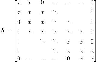
In general, the matrix can be represented in block tridiagonal form.

Another consequence of the Gram-Schmidt orthogonalization is that

Lemma:

Every finite dimensional inner-product space has an orthonormal basis.

Proof:

The proof is trivial. Just use Gram-Schmidt on any basis for that space and normalize. $\qquad \qquad \square$

A corollary of this is the following theorem.

Theorem:

Every finite dimensional inner product space is complete.

Recall that a space is complete is the limit of any Cauchy sequence from a subspace of that space must lie within that subspace.

Proof:

Let $\{\mathbf{u}_k\}$ be a Cauchy sequence of elements in the subspace $\mathcal{S}_n$ with $k = 1, \dots, \infty$ . Also let $\{\mathbf{e}_1, \mathbf{e}_2, \dots, \mathbf{e}_n\}$ be an orthonormal basis for the subspace $\mathcal{S}_n$ .

Then

\mathbf{u}_k = \sum_{j=1}^n \alpha_{kj}~\mathbf{e}_j

where

\alpha_{ki} = \langle \mathbf{u}_k, \mathbf{e}_i \rangle

By the Schwarz inequality

|\alpha_{ki} - \alpha_{pi}| = | \langle \mathbf{u}_k, \mathbf{e}_i \rangle - \langle \mathbf{u}_p, \mathbf{e}_i \rangle| \le \lVert\mathbf{u}_k - \mathbf{u}_p\rVert \rightarrow 0

Therefore,

\alpha_{ki} - \alpha_{pi} \rightarrow 0

But the $\alpha$ ~s are just numbers. So, for fixed $i$ , $\{\alpha_{ki}\}$ is a Cauchy sequence in $\mathbb{R}$ (or $\mathbb{C}$ ) and so converges to a number $\alpha_i$ as $k \rightarrow \infty$ , i.e.,

\lim_{k\rightarrow \infty} \mathbf{u}_k = \sum_{i=1}^n \alpha_i~\mathbf{e}_i

which is is the subspace $\mathcal{S}_n$ . $\qquad \qquad \square$

Spectral theory for matrices

Suppose $\boldsymbol{A}~\mathbf{x} = \mathbf{b}$ is expressed in coordinates relative to some basis $\boldsymbol{\varphi}_1, \boldsymbol{\varphi}_2, \dots, \boldsymbol{\varphi}_n$ , i.e.,

\boldsymbol{A}~\boldsymbol{\varphi}_j = \sum_i A_{ij}~\boldsymbol{\varphi}_i ~;~~ \mathbf{x} = \sum_i x_i~\boldsymbol{\varphi}_i ~;~~ \mathbf{b} = \sum_i b_i~\boldsymbol{\varphi}_i

Then

\boldsymbol{A}~\mathbf{x} = \boldsymbol{A}~\sum_j x_j~\boldsymbol{\varphi}_j = \sum_j x_j~(A~\boldsymbol{\varphi}_j) = \sum_{i,j} x_j~A_{ij}~\boldsymbol{\varphi}_i

So $\boldsymbol{A}~\mathbf{x} = \mathbf{b}$ implies that

\sum_{i,j} A_{ij}~x_j = b_i

Now let us try to see the effect of a change to basis to a new basis $\boldsymbol{\varphi}_1^{'}, \boldsymbol{\varphi}_2^{'}, \dots, \boldsymbol{\varphi}_n^{'}$ with

\boldsymbol{\varphi}_i^{'} = \sum_{j=1}^n C_{ji}~\boldsymbol{\varphi}_j

For the new basis to be linearly independent, $\mathbf{C}$ should be invertible so that

\boldsymbol{\varphi}_i = \sum_{j=1}^n C_{mj}^{-1}~\boldsymbol{\varphi}_m^{'}

Now,

\mathbf{x} = \sum_j x_j~\boldsymbol{\varphi}_j = \sum_{i,j} x_j~C_{ij}^{-1}~\boldsymbol{\varphi}_i^{'} = \sum_i x_i^{'}~\boldsymbol{\varphi}_i^{'}

Hence

x_i^{'} = C_{ij}^{-1}~x_j

Similarly,

b_i^{'} = C_{ij}^{-1}~b_j

Therefore

\boldsymbol{A}~\boldsymbol{\varphi}^{'} = \sum_{j=1}^n C_{ji}~\boldsymbol{A}~\boldsymbol{\varphi}_j = \sum_{j,k} C_{ji}~A_{kj}~\boldsymbol{\varphi}_k = \sum_{j, k, m} C_{ji}~A_{kj}~C_{mk}^{-1}~\boldsymbol{\varphi}_m^{'} = \sum_m A_{mi}^{'}~\boldsymbol{\varphi}_m^{'}

So we have

A_{mi}^{'} = \sum_{j, k} C_{mk}^{-1}~A_{kj}~C_{ji}

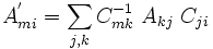
In matrix form,

\mathbf{x}^{'} = \mathbf{C}^{-1}~\mathbf{x} ~;~~ \mathbf{b}^{'} = \mathbf{C}^{-1}~\mathbf{b} ~;~~ \mathbf{A}^{'} = \mathbf{C}^{-1}~\mathbf{A}~\mathbf{C}

where the objects here are not operators or vectors but rather the matrices and vectors representing them. They are therefore basis dependent.

In other words, the matrix equation $\mathbf{A}~\mathbf{x} = \mathbf{b}$

Similarity transformation

The transformation

\mathbf{A}^{'} = \mathbf{C}^{-1}~\mathbf{A}~\mathbf{C}

is called a similarity transformation. Two matrices are equivalent or similar is there is a similarity transformation between them.

Diagonalizing a matrix

Suppose we want to find a similarity transformation which makes $\boldsymbol{A}$ diagonal, i.e.,

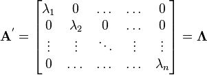
\mathbf{A}^{'} = \begin{bmatrix} \lambda_1 & 0 & \dots & \dots & 0 \\ 0 & \lambda_2 & 0 & \dots & 0 \\ \vdots & \vdots & \ddots & \vdots & \vdots \\ 0 & \dots & \dots & \dots & \lambda_n \end{bmatrix} = \boldsymbol{\Lambda}

Then,

\mathbf{A}~\mathbf{C} = \mathbf{C}~\mathbf{A}^{'} = \mathbf{C}~\boldsymbol{\Lambda}

Let us write $\mathbf{C}$ (which is a $n \times n$ matrix) in terms of its columns

\mathbf{C} = \begin{bmatrix} \mathbf{x}_1 & \mathbf{x}_2 & \dots & \mathbf{x}_n \end{bmatrix}

Then,

\mathbf{A}~ \begin{bmatrix} \mathbf{x}_1 & \mathbf{x}_2 & \dots & \mathbf{x}_n \end{bmatrix} = \begin{bmatrix} \mathbf{x}_1 & \mathbf{x}_2 & \dots & \mathbf{x}_n \end{bmatrix}~\boldsymbol{\Lambda} = \begin{bmatrix} \lambda_1~\mathbf{x}_1 & \lambda_2~\mathbf{x}_2 & \dots & \lambda_n~\mathbf{x}_n \end{bmatrix}

i.e.,

\mathbf{A}~\mathbf{x}_i = \lambda_i~\mathbf{x}_i

The pair $(\lambda, \mathbf{x})$ is said to be an eigenvalue pair if $\mathbf{A}~\mathbf{x} = \lambda~\mathbf{x}$ where $\mathbf{x}$ is an eigenvector and $\lambda$ is an eigenvalue.

Since $(\mathbf{A} - \lambda~\mathbf{I}) = \mathbf{0}$ this means that $\lambda$ is an eigenvalue if and only if

\det(\mathbf{A} - \lambda~\mathbf{I}) = \mathbf{0}

The quantity on the left hand side is called the characteristic polynomial and has $n$ roots (counting multiplicities).

In $\mathbb{C}$ there is always one root. For that root $\mathbf{A} - \lambda~\mathbf{I}$ is singular, i.e., there always exists at least one eigenvector.

We will delve a bit more into the spectral theory of matrices in the next lecture.

Resource type: this resource contains a lecture or lecture notes.

Action required: please create Category:Applied linear operators and spectral methods/Lectures and add it to Category:Lectures.

This article is issued from Wikiversity - version of the Wednesday, June 04, 2008. The text is available under the Creative Commons Attribution/Share Alike but additional terms may apply for the media files.