Applied linear operators and spectral methods/Lecture 2
< Applied linear operators and spectral methodsNorms in inner product spaces
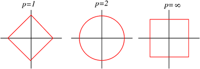
Inner product spaces have  norms which are defined as

When  , we get the
  norm
norm

When  , we get the
  norm
norm

In the limit as  we get the
  norm or the sup norm

The adjacent figure shows a geometric interpretation of the three norms.
 Geomtric interpretation of various norms |
If a vector space has an inner product then the norm

is called the induced norm. Clearly, the induced norm is nonnegative and zero only
if  . It is also linear under multiplication by a positive vector. You can
think of the induced norm as a measure of length for the vector space.
. It is also linear under multiplication by a positive vector. You can
think of the induced norm as a measure of length for the vector space.
So useful results that follow from the definition of the norm are discussed below.
Schwarz inequality
In an inner product space

Proof
This statement is true if  .
.
If  we have

Now

Therefore,

Let us choose  such that it minimizes the left hand side above. This value is
clearly
such that it minimizes the left hand side above. This value is
clearly

which gives us
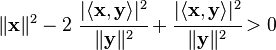
Therefore,

Triangle inequality
The triangle inequality states that

Proof

From the Schwarz inequality

Hence

Angle between two vectors
In  or
or  we have

So it makes sense to define  in this way for any real vector space.
We then have

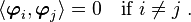
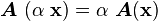
Orthogonality
In particular, if  we have an analog of the Pythagoras theorem.

In that case the vectors are said to be orthogonal.
If  then the vectors are said to be orthogonal even in a complex
vector space.
then the vectors are said to be orthogonal even in a complex
vector space.
Orthogonal vectors have a lot of nice properties.
Linear independence of orthogonal vectors
- A set of nonzero orthogonal vectors is linearly independent.
If the vectors  are linearly dependent

and the are orthogonal, then taking an inner product with  gives
gives

since
Therefore the only nontrivial case is that the vectors are linearly independent.
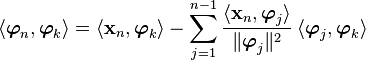
Expressing a vector in terms of an orthogonal basis
If we have a basis 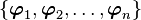 and wish to express a
vector
and wish to express a
vector  in terms of it we have
The problem is to find the  s.
s.
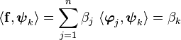
If we take the inner product with respect to , we get
In matrix form,

where  and
and  .
.
Generally, getting the s involves inverting the  matrix
  , which is an identity matrix
  , because
  , where
  is the Kronecker delta.
Provided that the s are orthogonal then we have
and the quantity
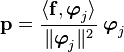
is called the projection of onto .
Therefore the sum
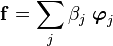
says that is just a sum of its projections onto the orthogonal basis.
 Projection operation. |
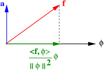
Let us check whether  is actually a projection. Let
Then,
Therefore  and
and  are indeed orthogonal.
Note that we can normalize by defining

Then the basis  is called an orthonormal basis.
It follows from the equation for that

and
You can think of the vectors  as orthogonal unit vectors in
an
as orthogonal unit vectors in
an  -dimensional space.
Biorthogonal basis
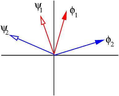
However, using an orthogonal basis is not the only way to do things. An alternative that is useful (for instance when using wavelets) is the biorthonormal basis.
The problem in this case is converted into one where, given any basis
, we want to find another set
of vectors  such that
In that case, if
it follows that
So the coefficients  can easily be recovered. You can see a schematic
of the two sets of vectors in the adjacent figure.
can easily be recovered. You can see a schematic
of the two sets of vectors in the adjacent figure.
 Biorthonomal basis |
Gram-Schmidt orthogonalization
One technique for getting an orthogonal baisis is to use the process of Gram-Schmidt orthogonalization.
The goal is to produce an orthogonal set of vectors
given a linearly independent set
 .
.
We start of by assuming that  . Then
  is given by
subtracting the projection of
is given by
subtracting the projection of  onto
onto  from , i.e.,
Thus is clearly orthogonal to . For  we use
More generally,
If you want an orthonormal set then you can do that by normalizing the orthogonal set of vectors.
We can check that the vectors are indeed orthogonal by induction.
Assume that all  are orthogonal for some
  . Pick
 . Then
Now 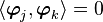 unless
  . However, at ,
 because the two remaining terms cancel out. Hence
the vectors are orthogonal.
because the two remaining terms cancel out. Hence
the vectors are orthogonal.
Note that you have to be careful while numerically computing an orthogonal basis using the Gram-Schmidt technique because the errors add up in the terms under the sum.
Linear operators
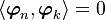
The object  is a linear operator from
  onto if

A linear operator satisfies the properties
 .
. .
.
Note that is independent of basis. However, the action of on a basis
determines completely since
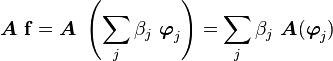
Since  we can write
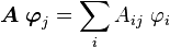
where  is the matrix representing the operator in the basis
.
is the matrix representing the operator in the basis
.
Note the location of the indices here which is not the same as what we get in matrix
multiplication. For example, in  , we have

We will get into more details in the next lecture.
| | Resource type: this resource contains a lecture or lecture notes. |
| | Action required: please create Category:Applied linear operators and spectral methods/Lectures and add it to Category:Lectures. |