Applied linear operators and spectral methods/Lecture 1
< Applied linear operators and spectral methodsLinear operators can be thought of as infinite dimensional matrices. Hence we can use well known results from matrix theory when dealing with linear operators. However, we have to be careful. A finite dimensional matrix has an inverse if none of its eigenvalues are zero. For an infinite dimensional matrix, even though all the eigenvectors may be nonzero, we might have a sequence of eigenvalues that tend to zero. There are several other subtleties that we will discuss in the course of this series of lectures.
Let us start off with the basics, i.e., linear vector spaces.
Linear Vector Spaces ( )
)
Let be a linear vector space.
Addition and scalar multiplication
Let us first define addition and scalar
multiplication in this space. The addition operation acts completely in
while the scalar multiplication operation may involved multiplication either
by a real (in  ) or by a complex number (in
  ). These
operations must have the following closure properties:
). These
operations must have the following closure properties:
- If
 then
then  .
. - If
 (or ) and
  then
then  .
.
And the following laws must hold for addition
 =
=  Commutative law.
 =
=  Associative law.
 such that
  Additive identity.
 such that
  Additive inverse.
For scalar multiplication we have the properties
 .
. .
. .
. .
. .
.
Example 1:  tuples
The tuples 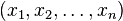 with
with

form a linear vector space.
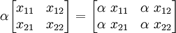
Example 2: Matrices
Another example of a linear vector space is the set of  matrices
with addition as usual and scalar multiplication, or more generally
matrices
with addition as usual and scalar multiplication, or more generally  matrices.
Example 3: Polynomials
The space of -th order polynomials forms a linear vector space.
Example 4: Continuous functions
The space of continuous functions, say in ![[0, 1]](../I/m/ccfcd347d0bf65dc77afe01a3306a96b.png) , also forms a linear vector
space with addition and scalar multiplication defined as usual.
, also forms a linear vector
space with addition and scalar multiplication defined as usual.
Linear Dependence
A set of vectors  are said to be linearly
dependent if
are said to be linearly
dependent if 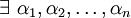 not all zero such that

If such a set of constants  do not exists
then the vectors are said to be linearly independent.
do not exists
then the vectors are said to be linearly independent.
Example
Consider the matrices
These are linearly dependent since  .
.
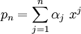
Span
The span of a set of vectors  is the set of all vectors that are
linear combinations of the vectors
is the set of all vectors that are
linear combinations of the vectors  . Thus

where

as vary.
Spanning set
If the span = then  is said to be a spanning set.
Basis
If is a spanning set and its elements are linearly independent then we call
it a basis for . A vector in has a unique representation as a
linear combination of the basis elements. why is it unqiue?
Dimension
The dimension of a space is the number of elements in the basis. This is
independent of actual elements that form the basis and is a property of .
Example 1: Vectors in 
Any two non-collinear vectors is a basis for
because any other vector in can be expressed as a linear
combination of the two vectors.
Example 2: Matrices
A basis for the linear space of matrices is
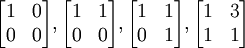
Note that there is a lot of nonuniqueness in the choice of bases. One important skill that you should develop is to choose the right basis to solve a particular problem.
Example 3: Polynomials
The set 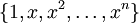 is a basis for polynomials of degree .
Example 4: The natural basis
A natural basis is the set 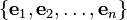 where the
  th
entry of
th
entry of  is
is
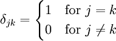
The quantity  is also called the Kronecker delta.
Inner Product Spaces
To give more structure to the idea of a vector space we need concepts such as magnitude and angle. The inner product provides that structure.
The inner product generalizes the concept of an angle and is defined as a function

with the properties
 overbar indicates complex conjugation.
 Linear with respect to scalar multiplication.
 Linearity with respect to addition.
 if
if  and
and  if and only if
  .
.
A vector space with an inner product is called an inner product space.
Example 1:

Example 2: Discrete vectors
In  with
with  and
and
 the Eulidean norm is given by

With  the standard norm is

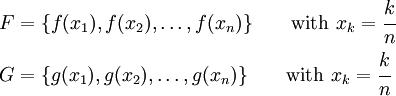
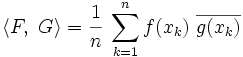
Example 3: Continuous functions
For two complex valued continuous functions  and
and  in
we could approximately represent them by their function values at
equally spaced points.
in
we could approximately represent them by their function values at
equally spaced points.
Approximate and by
With that approximation, a natural norm is
Taking the limit as  (show this)

If we took non-equally spaced yet smoothly distributed points we would get
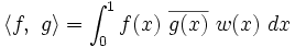
where  is a smooth weighting function (show this).
There are many other inner products possible. For functions that are not only continuous but also differentiable, a useful norm is
![\langle f,~g\rangle = \int_0^1 \left[f(x)~\overline{g(x)} +
f^{'}(x)~\overline{g^{'}(x)}\right]~dx](../I/m/fc4620a8e9efed1703e22b14f2a8da1d.png)
We will continue further explorations into linear vector spaces in the next lecture.
| | Resource type: this resource contains a lecture or lecture notes. |
| | Action required: please create Category:Applied linear operators and spectral methods/Lectures and add it to Category:Lectures. |