Advanced Classical Mechanics/Continuum Mechanics
< Advanced Classical MechanicsWe can extend the formalism of Lagrangian mechanics to cover the motion of continuous materials: membranes, strings and fields.
Deriving the Lagrange Equations of a Continuum
We saw for a string that the potential and kinetic energy can be written as a integral over the length of the string.
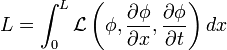
where  is called the Lagrangian density.
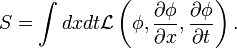
The Action
Let's write out the action
We would like to find the function  that minimizes the action, so we
let
that minimizes the action, so we
let  and calculate
![\delta S = \int dx dt \left [ \left .\frac{\partial {\mathcal L}}{\partial \phi} \right |_{\phi_0}
\eta +
\left .\frac{\partial {\mathcal L}}{\partial
\left ( \frac{\partial \phi}{\partial x}\right )} \right |_{\phi_0}
\frac{\partial \eta}{\partial x} +
\left . \frac{\partial {\mathcal L}}{\partial
\left ( \frac{\partial \phi}{\partial t}\right )} \right |_{\phi_0}
\frac{\partial \eta}{\partial t}
\right ].](../I/m/adfb4dd749a0df53f37e614f0534aade.png)
Let integrate the last two items by parts and drop the boundary term because we assume that the value of  vanishes on the boundary, we get
![\delta S = \int dx dt \eta \left [ \left .\frac{\partial {\mathcal L}}{\partial \phi} \right |_{\phi_0}
-
\frac{d}{dx} \left .\frac{\partial {\mathcal L}}{\partial
\left ( \frac{\partial \phi}{\partial x}\right )} \right |_{\phi_0}
-
\frac{d}{dt}
\left . \frac{\partial {\mathcal L}}{\partial
\left ( \frac{\partial \phi}{\partial t}\right )} \right |_{\phi_0}
\right ].](../I/m/14f3bd2319f497b588fd434dcc4af17c.png)
Lagrange's Equations
Because the function is completely arbitrary then for the value of  to vanish, the integrand itself must vanish and we obtain the Lagrange equation for a field in one spatial dimension:
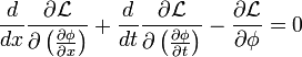
that the actual motion must satify.
Each new dimension that the field lives in adds a new term of the form

to the equations of motion.
Examples
Electrostatics
Let's do an example of an electric field with a bunch of charges around. The energy density of an electric field with charges around is
We would like to minimize the integral of  over a volume so it is natural to take
  . We have
![{\mathcal L} = \frac{\epsilon_0}{2} \left [ \left ( \frac{\partial \phi}{\partial x} \right )^2 + \left ( \frac{\partial \phi}{\partial y} \right)^2 \right ] + \rho \phi](../I/m/67afdd53d1be4b4849caf8e03a1d5463.png)
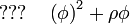
and Lagrange's equations are
A String
As a problem toward the beginning of the term, you found that the potential energy of a string could be given by
where  is the string tension.
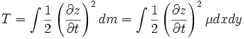
We can also write the kinetic energy of the string as an integral
where  , the mass per unit length of the string. We can combine these two expressions to get the Langrangian density
![{\mathcal L} = \frac{1}{2} \left [ \mu \left ( \frac{\partial z}{\partial t} \right )^2 - \lambda \left ( \frac{\partial z}{\partial x} \right )^2 \right ].](../I/m/908ba8434950a5bbcbbde59a733e1076.png)
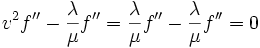
Now let's apply Lagrange's equations to this Lagrangian density,
We can find a solution to this equation of the form,
 where
where  . Let's substitute this into the equation to get
This solution is a wave travelling in the positive or negative x-direction. The function f can take any form whatsoever and it always travels at the same speed. This type of wave is called a 'simple wave'.
The Discrete Fourier Transform
When a string vibrates it causes the air around it to vibrate as well; these vibrations travel through the air as waves that we can detect with the acoustic spectrometers attached to the sides of our heads. Our ears are sensitive to the pitch or frequency of the sound that the string produces so it is natural to look at the waves along a string as a sum of waves of a particular frequency, so we have
 where φ is the phase of the wave.
Let's substitute this into the equation of motion to get
 so
so
 and
and
Now we must apply the boundary conditions of the string. Specifically, we have  so
so
where n is an integer so we have a formula for the frequency of the wave in terms of the form of the oscillation along the string
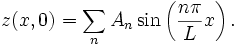
The general solution will allow a sum of different frequencies so
Let's suppose that we pluck the string so that a t=0, the string is not straight but it is not moving either, so we have  in the formula above, and we get
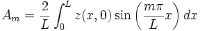
We would like to find the coefficients  that tell us what pitches the string will emit when it is released.
Let's take the integral of both sides times  to get

![= \int_0^L \sum_n \frac{A_n}{2} \left [ \cos \left ( \frac{(n+m)\pi}{L} x \right )
+ \cos\left ( \frac{(n-m)\pi}{L} x \right ) \right ] dx = \int_0^L \frac{A_m}{2} d x = \frac{A_m L}{2}.](../I/m/b18fcf9e87ea77922086a33e69152992.png)
Rearranging we have
which defines the discrete Fourier transform.
A Membrane
As a problem toward the beginning of the term, you found that the potential energy of a string could be given by
![V = \int \frac{1}{2} \lambda \left [ \left ( \frac{\partial z}{\partial x} \right )^2 + \left ( \frac{\partial z}{\partial y} \right )^2\right ] dx dy](../I/m/fa0805a01eff3f1002bae344f3548534.png)
where is the surface tension.
We can also write the kinetic energy of the membrane as an integral
where  , the mass per unit area of the membrane. We can combine these two expressions to get the Langrangian density
![{\mathcal L} = \frac{1}{2} \left [ \mu \left ( \frac{\partial z}{\partial t} \right )^2 - \lambda \left [ \left ( \frac{\partial z}{\partial x} \right )^2 + \left ( \frac{\partial z}{\partial y} \right )^2 \right ] \right ] = \frac{1}{2} \left [ \mu \left ( \frac{\partial z}{\partial t} \right )^2 - \lambda \left ( \nabla z \right )^2 \right ]](../I/m/dce22bcf4ef2a8176cdae6da52b50eda.png)
If we apply Lagrange's equations we obtain,
Different Coordinates
The value of the action does not depend on the coordinates that you use, but as we shall see the Lagrangian density does. First let's write the action using Cartesian coordinates
![S = \int dx dy {\mathcal L} = \int dx dy = \frac{1}{2} \left [ \mu \left ( \frac{\partial z}{\partial t} \right )^2 - \lambda \left ( \nabla z \right )^2 \right ].](../I/m/44c52f8d387a8a2ad9da78e402ef16a2.png)
Sometimes it is useful to use polar coordinates for a circular drum perhaps. Here the action is
![S = \int dr d\theta {\mathcal L} = \int dr d\theta r \frac{1}{2} \left [ \mu \left ( \frac{\partial z}{\partial t} \right )^2 - \lambda \left ( \nabla z \right )^2 \right ].](../I/m/23477de97ecdb09d6db8249a25d7fb43.png)
Notice that an r appears in front of the "Cartesian" Lagrangian density. This is just so the units work out, so we find that
In both coordinate systems the action has the same units but the Lagrangian density does not. We also need to rewrite the spatial derivatives in polar coordinates to get
![{\mathcal L}_{\rm polar}
= \frac{1}{2} r \left [ \mu \left ( \frac{\partial z}{\partial t} \right )^2 - \lambda \left ( \nabla z \right )^2 \right ]
= \frac{1}{2} r \left [ \mu \left ( \frac{\partial z}{\partial t} \right )^2 - \lambda \left [
\left ( \frac{\partial z}{\partial r} \right )^2 + \left ( \frac{1}{r} \frac{\partial z}{\partial \theta} \right )^2\right ] \right ]](../I/m/a48b4f0d28339256712eefd083534591.png)
If we apply the Lagrange equations we find that the Lagrange density depends explicitly on the coordinate r. We obtain,
and divide both sides by r to get
![\mu \frac{\partial^2 z}{\partial t^2} - \lambda \left [ \frac{1}{r} \frac{d}{dr} \left ( r \frac{\partial z}{\partial r} \right ) + \frac{1}{r^2} \frac{\partial^2 z}{\partial \theta^2} \right ] = 0](../I/m/a64bccf01c917eb9ce26b580480c5347.png)
or using the definition of the Laplacian in cylindrical coordinates we get
Solutions to the Two-Dimensional Wave Equation
When analyzing a drum or something with boundary conditions, it is natural to look for solutions to these equations
with the form
 in Cartesian coordinates,
 in cylindrical coordinates, or
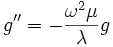
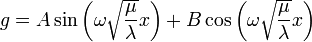
 Generally you can pick the function g to vary harmonically in time and the solutions to the spatial dependence
are known as harmonics. In Cartesian coordinates we get sines and cosines (the harmonic functions). In cylidrical coordinates, we get sines and cosines in the
Generally you can pick the function g to vary harmonically in time and the solutions to the spatial dependence
are known as harmonics. In Cartesian coordinates we get sines and cosines (the harmonic functions). In cylidrical coordinates, we get sines and cosines in the  -direction and Bessel functions in the radial direction. If your drum is the surface of a sphere, the solutions are called spherical harmonics: sines and cosines in the
  direction and polynomials of
  in the other direction.
A Slung Slinky
As a final example we will study a slinky hanging from a horizontal surface and the waves that can propagate along it. Let's first draw a picture to show what we are talking about
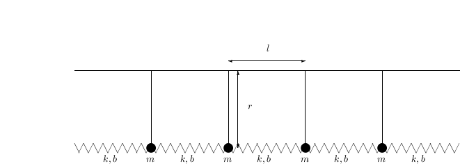
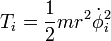
Let's use the variable  to denote the angle that each pendulum makes with the vertical. Also let's restrict ourselves to the small-angle approximation. We can write the kinetic energy of each mass as
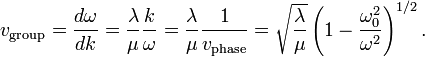
There are two sources of potential energy: gravity and the springs. The expression for gravity is straightforward we have
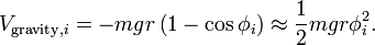
The potential energy of the springs is a bit more complicated. First, we have to come up with a convention so that we don't double count the springs. Let's identify a spring with the mass to its left so we have
![V_{{\rm spring},i} = \frac{1}{2} k \left \{ r \left[ \left ( \frac{b}{r} + \sin\phi_{i+1} - \sin\phi_i \right )^2 + \left (\cos \phi_{i+1}-\cos\phi_i\right)^2 \right ]^{1/2} - l \right \}^2](../I/m/384a36bb9833166ad1bbab286d4027f0.png)
Now let's take the small-angle approximation,

We can simplify this further. The first term is a constant; let's drop it. The second term sums to zero when one combines the contribution from every spring. The final term is
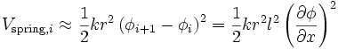
where we have replaced with  .
.
The Lagrange density is given by
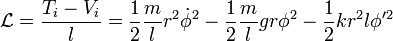
The Klein-Gordon Equation
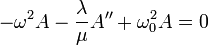
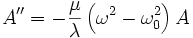
Let's apply Lagrange's equations to the Lagrange density to get the following equation of motion
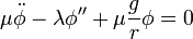
where  and
and  . This equation of motion is very similar to that of the stretched string but there is an extra term. Let's divide both sides by
  to get
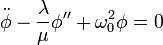
where  is the natural frequency of the hanging masses. This is known as the Klein-Gordon equation, and it describes the evolution of massive scalar field.
If we let the spring constant
is the natural frequency of the hanging masses. This is known as the Klein-Gordon equation, and it describes the evolution of massive scalar field.
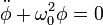
If we let the spring constant  go to zero, then goes to zero as well and we have the simple equation for a pendulum.
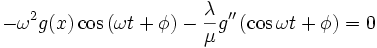
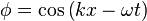
To get an appreciation for the solutions, let's substitute a harmoncally varying wave
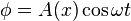
to get
 and
and
If the frequency of the wave  is greater than the natural frequency of the pendulum, the wave varies sinusoidally in space as well as time (it propagates along the slinky). On the other hand, low-frequency waves are damped, so the slung slinky acts as a high-pass filter.
The form of the equation above encourages us to use solutions of the form
with the dispersion relation
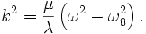
Phase Velocity
Again we see that when  things get a bit funny. We can define the phase velocity of the wave
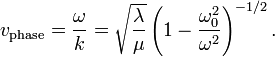
This measures the speed at which the crest of a wave of a particular frequency passes by.
Group Velocity
Let's say that we want to send a signal down the slinky. How long fast will the signal travel? Specifically, we would like to displace the end of the slinky back and forth and watch the compression travel along the spring.
We could naturally think of a signal as the sum of two waves of a single frequency.
![A (x, t) = \cos \left [ \left ( k + \Delta k \right ) x - \left ( \omega + \Delta \omega \right ) t \right ]
+ \cos \left [ \left ( k - \Delta k \right ) x - \left ( \omega - \Delta \omega \right ) t \right ].](../I/m/ed426e6afe25b403fa2b34ae29e3be8e.png)
Using some trignometric identites we see that this is just an amplitude-modulated wave

The amplitude modulation is a wave that travels on top of the carrier wave at a speed of
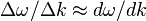 for narrow bandwidth.
The group velocity measures the speed of a "wave packet" or how long a signal takes to travel along the slinky
If we think about the wave described above in more detail, we have a rapid back-and-forth oscillation that travels at the phase velocity and on top of it a variation in the amplitude of the rapid oscillation. If we ignored the frequency of the pendulums (taking  or
or  ), these two variations would travel at the speed
  and one would simply see a pattern travelling at a constant speed along the slinky.
Hanging the slinky introduces dispersion, this means that the pattern generally changes as it travels along the slinky.
The Sine-Gordon or Pendulum Equation
The slung Slinky is related to another important equation of physics. Let's take the exact expression for the gravitational potential energy
The new Lagrange density is given by

and the equation of motion is
This is known as the sine-Gordon equation (those physicists are really good punsters). This equation is no longer linear in the variable
 so it is much more difficult to solve than the Klein-Gordon equation. Specifically, we expect that the velocity of the wave will depend not only on the frequency but also the amplitude.
We can define our scale of time ( ) and distance (
 ) so that the equation takes the simpler form

Let's look for solutions that have a fixed pattern travelling at a fixed velocity. This was not possible (except for a monochromatic wave) for the Klein-Gordon equation because of the dispersion. Here we have dispersion and non-linearity. Let's use
to get
so
Here the value of velocity depends on the amplitude of the wave,  for an amplitude of 0.01,
  for an amplitude of 1 and 1.64 for an amplitude of 2.
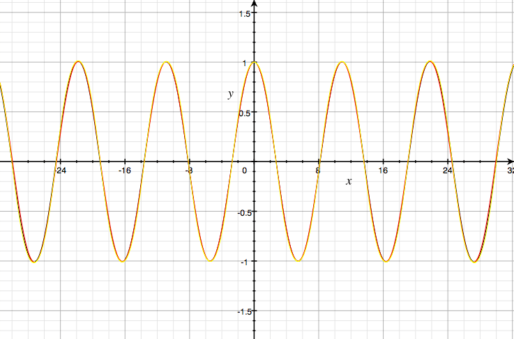
Solitons
The solutions above are strictly periodic, but we can also find waves that travel at velocities less than one that are not periodic (i.e. they are solitary waves or solitons).
The wider waves have amplitudes closer to  and velocities closer to zero. The speed of the solitons are 0.1, 0.5, 0.8 and 0.9 from widest to narrowest and the amplitudes range from 6.17 down to 6.11.
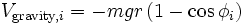
The differential equation actually has a simple solution as well. It is called the "kink" solution
![\phi = 4 \tan^{-1} \left [ \exp \left ( \frac{x-vt}{\sqrt{1-v^2}} \right ) \right ]](../I/m/387eda69da17af52b46985c566d2fe90.png)
The speed at which the kink travels depends on the maximum slope of the kink.
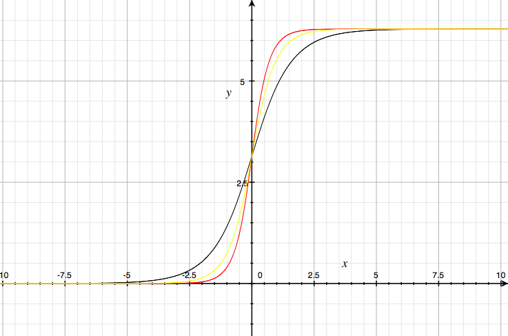
The steepest slope travels at  ; then we have 0.8 and zero (a frozen kink).