Adams-bashforth and Adams-moulton methods
| |
Subject classification: this is a mathematics resource . |
Definitions
Linearmultistepmethodsareusedforthenumericalsolutionofordinarydifferentialequations, inparticularthe initial value problem

The Adams-Bashforth methods and Adams-Moulton methods are described on the Linear multistep method page.
Derivation
There are (at least) two ways that can be used to derive the Adams-Bashforth methods and Adams-Moulton methods. We will demonstrate the derivations using polynomial interpolation and using Taylor's theorem for the two-step Adams-Bashforth method.
Derive the two-step Adams-bashforth method by using polynomial interpolation
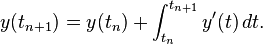
From the w:Fundamental theorem of Calculus we can get
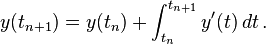
(1 )
Set
-
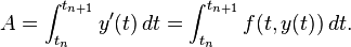
(2 )
To get the value of  , we can use an interpolating polynomial
  as an approximation of
  .
The interpolation polynomial in the Lagrange form is a linear combination
.
The interpolation polynomial in the Lagrange form is a linear combination
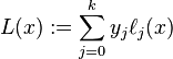
where
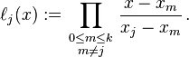
Then the interpolation can be
Thus, (2 ) becomes
-

(3 )
Integrating and simplifying, the right hand side of equation (3 ) becomes
Since  ,
,  and
and  are equally spaced, then
  .
Therefore, the value of is
.
Therefore, the value of is
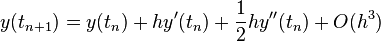
Putting this value back to (1 ) yields

Thus, the equation
 is the two-step Adams-Bashforth method.
Derive the two-step Adams-Bashforth method by using Taylor's theorem
To simplify, let's set  .
Then the general form of Adams-Bashforth method is
.
Then the general form of Adams-Bashforth method is
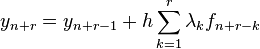
(4 )
where  .
For the two-step Adams-Bashforth method, let's set
.
For the two-step Adams-Bashforth method, let's set 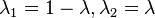 . Then (4
) becomes
. Then (4
) becomes
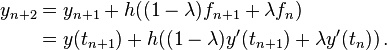
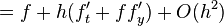
By using Taylor's theorem, expand  at to get

Thus, the simplified form is
-

(5 )
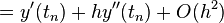
Expanding  at
at  yields
-

(6 )
Subtracting (5
) from (6
) and then requiring the h^2 term to cancel makes  .
The two-step Adams-Bashforth method is then
.
The two-step Adams-Bashforth method is then
Since

the local truncation error is of order  and thus the method is second order.
(See w: Linear multistep method#Consistency and order and w:Truncation error)
and thus the method is second order.
(See w: Linear multistep method#Consistency and order and w:Truncation error)
Exercises
1. Derive three-step Adams-Bashforth method by using polynomial interpolation
Solution:
The initial problem is  Then we can get:
-
(8 )
let's set:
-
(9 )
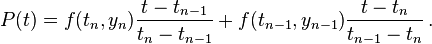
Then,we can use P(t) as an interpolation of f(t,y(t)). To derive the three-step Adams-bashforth method, the interpolation polynomial is:

Since  , , and are equally spaced, then
 .
.
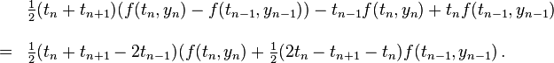
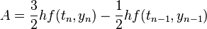
So the integral of each part of P(t) is :
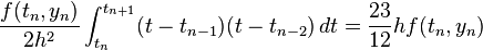


Thus the approximate value of A is

Put this value back to (8 )

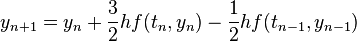
Thus, the three-step Adams-Bashforth method is

2. Derive the second-order Adams-Moulton method by using Taylor's theorem
Solution:
To simplify, note  to represent
 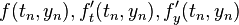 .From Taylor expansion of the binary function (w:Taylor's theorem):
![f_{n+1}=f(t_{n+1},y_{n+1})=f+hf'_{t}+f'_{y}(y_{n+1}-y_{n})+O[h^2+(y_{n+1}-y_{n})^2]](../I/m/c7f48fcfda733d9cfcd60cfa53012b7e.png)
Then by using:
-

(10 )
can get:

Therefore, simplify this equation to get:
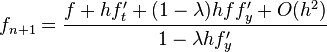
![=[f+hf'_{t}+(1-\lambda)hff'_{y}+O(h^2)][1+\lambda hf'_{y}+O(h^2)]](../I/m/5c2e42ca8553939fd88f9ed7d33f92b1.png)
Thus, subtitute  into (10
):
into (10
):
![y_{n+1}=y_{n}+h[(1-\lambda)f_{n}+\lambda f_{n+1}]](../I/m/c7d6a284a702cd5830daf516fa9943f4.png)

Combining the equation:

and Taylor expansion:
can get  . Therefore, the second-order Adams-moulton method is:
Predictor–corrector method
To solve an ordinary differential equation (ODE), a w:Predictor–corrector method is an algorithm that can be used in two steps. First, the prediction step calculates a rough approximation of the desired quantity, typically using an explicit method. Second, the corrector step refines the initial approximation using another means, typically an implicit method.
Here mainly discuss about using Adams-bashforth and Adams-moulton methods as a pair to contruct a predictor–corrector method.
Example: Adams predictor–corrector method
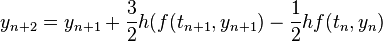
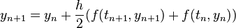
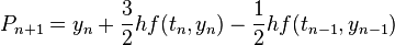
Let's start from the two-step Adams method. The prediction step is to use two-step Adams-bashforth:
Then, by using two-step Adams-moulton the corrector step can be:

Also, by using four-step Adams-bashforth and Adams-moulton methods together, the predictor-corrector formula is:

Note, the four-step Adams-bashforth method needs four initial values to start the calculation. It needs to use other methods, for example Runge-Kutta, to get these initial values.
matlab program
The four-step Adams predictor-corrector matlab program code is
function [x y]=maadams4(dyfun,xspan,y0,h)
% use four-step Adams predictor-corrector method to solve an ODE y'=f(x,y), y(x0)=y0
% inputs: dyfun -- the function f(x,y), as an inline
% xspan -- the interval [x0,xn]
% y0 -- the initial value
% h -- the step size
% output: x, y -- the node and the value of y
x=xspan(1):h:xspan(2);
% use Runge-Kutta method to get four initial values
[xx,yy]=marunge(dyfun,[x(1),x(4)],y0,h);
y(1)=yy(1);y(2)=yy(2);
y(3)=yy(3);y(4)=yy(4);
for n=4:(length(x)-1)
p=y(n)+h/24*(55*feval(dyfun,x(n),y(n))-59*feval(dyfun,x(n-1),y(n-1))+37*feval(dyfun,x(n-2),y(n-2))-9*feval(dyfun,x(n-3),y(n-3)));
y(n+1)=y(n)+h/24*(9*feval(dyfun,x(n+1),p)+19*feval(dyfun,x(n),y(n))-5*feval(dyfun,x(n-1),y(n-1))+feval(dyfun,x(n-2),y(n-2)));
end
x=x';y=y';
The matlab code of Runge-Kutta method is:
function [x y]=marunge(dyfun,xspan,y0,h)
x=xspan(1):h:xspan(2);
y(1)=y(0);
for n=1:(length(x)-1)
 k1=feval(dyfun,x(n),y(n));
 k2=feval(dyfun,x(n)+h/2,y(n)+h/2*k1);
 k3=feval(dyfun,x(n)+h/2,y(n)+h/2*k2);
 k4=feval(dyfun,x(n+1),y(n)+h*k3);
 y(n+1)=y(n)+h*(k1+2*k2+2*k3+k4)/6;
end
x=x';y=y'
References
- http://www-users.cselabs.umn.edu/classes/Spring-2011/csci5302/Notes/Multistep_ABM.pdf
- http://www.phy.ornl.gov/csep/ode/node12.html