Transportation Geography and Network Science/Centrality
< Transportation Geography and Network ScienceSummary
There are a variety of networks in transportation geography, such as the airline networks, road networks, and canal networks. One important question is how to measure these networks. If we focus on properties of the nodes, the questions can be: how important are certain nodes? And how to quantify their importance?
Centrality measures are often used to measure a node's importance. There are three major categories: degree centrality, closeness centrality, and betweenness centrality.
Degree centrality
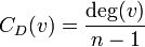
Degree centrality measures the importance of a node by the number of edges (degree) the node has. The idea is that a node with more edges is more important. Mathematically, for node j, its degree centrality is calculated as the number of its degrees divided by n-1, where n is the total number of edges in the graph.
Closeness centrality
Closeness centrality measures the importance of a node by its geodesic distance to other nodes. The idea is that the closer a node is to other nodes, the important the node is. Mathematically it is calculated as the reciprocal of the sum of geodesic distances to all other nodes [1].
Betweenness centrality
Betweenness centrality measures the importance of a node by its proportion of paths between other nodes. The idea is that a node that plays the roles of connecting more other nodes is more important. Mathematically, the betweenness centrality of node j is calculated as the proportion of shortest paths from one node s to another node node t that passes through j.
A thought experiment
Which centrality measures will you use for answering the following questions? [2].
- If I need to recruit 10 people for my newly found organization, whom should I consider?
- If I am to pass on a message to three people in this network so that they in turn convey it to their friends and so on. Which three people should I select?
- If I am to rank all my friends based on how "central" they are in this network, how would I go about?
- If I am to nominate a leader for this team of 500, whom should I pick?
Technical Discussion
Adapted from Wikipedia article on Centrality
Within w:graph theory and w:network analysis, there are various measures of the centrality of a vertex within a graph that determine the relative importance of a vertex within the graph (for example, how important a person is within a w:social network, or, in the theory of w:space syntax, how important a room is within a building or how well-used a road is within an w:urban network).
There are four measures of centrality that are widely used in network analysis: degree centrality, betweenness, closeness, and eigenvector centrality. For a review as well as generalizations to weighted networks, see Opsahl et al. (2010)[3].
Degree centrality
The first, and simplest, is degree centrality. Degree centrality is defined as the number of links incident upon a node (i.e., the number of ties that a node has). Degree is often interpreted in terms of the immediate risk of node for catching whatever is flowing through the network (such as a virus, or some information). If the network is directed (meaning that ties have direction), then we usually define two separate measures of degree centrality, namely w:indegree and w:outdegree. Indegree is a count of the number of ties directed to the node, and outdegree is the number of ties that the node directs to others. For positive relations such as friendship or advice, we normally interpret indegree as a form of popularity, and outdegree as gregariousness.
For a graph  with n vertices, the degree centrality
  for vertex
  is:
is:
Calculating degree centrality for all nodes  in a graph takes
  in a dense w:adjacency matrix representation of the graph, and for edges
  in a graph takes
  in a w:sparse matrix representation.
The definition of centrality can be extended to graphs. Let  be the node with highest degree centrality in
  . Let
. Let  be the
  node connected graph that maximizes the following quantity (with
  being the node with highest degree centrality in
  ):
):
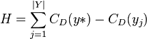
Then the degree centrality of the graph is defined as follows:
![C_D(G)= \frac{\displaystyle{\sum^{|V|}_{i=1}{[C_D(v*)-C_D(v_i)]}}}{H}](../I/m/755c1a4f0f1f33c8fbb345d7c4187c7d.png)
 is maximized when the graph contains one node that is connected to all other nodes and all other nodes are connected only to this one central node (a w:star graph). In this case
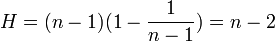
so the degree centrality of reduces to:
![C_D(G)= \frac{\displaystyle{\sum^{|V|}_{i=1}{[C_D(v*)-C_D(v_i)]}}}{n-2}](../I/m/626fe0293c646871eb39e7a637811ec0.png)
Betweenness centrality
Betweenness is a centrality measure of a vertex within a graph (there is also edge betweenness, which is not discussed here). Vertices that occur on many shortest paths between other vertices have higher betweenness than those that do not.
For a graph with n vertices, the betweenness  for vertex is computed as follows:
1. For each pair of vertices (s,t), compute all shortest paths between them.
2. For each pair of vertices (s,t), determine the fraction of shortest paths that pass through the vertex in question (here, vertex v).
3. Sum this fraction over all pairs of vertices (s,t).
Or, more succinctly:[4]
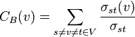
where  is the number of shortest paths from s to t, and
  is the number of shortest paths from s to t that pass through a vertex v. This may be normalized by dividing through the number of paths that are examined, which is
 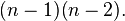 For undirected graphs, only one of the directions between each pair of vertices has to be examined, so only
 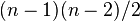 paths in total, which is also the number of pairs of vertices not including v. For example, in an undirected star graph, the center vertex (which is contained in every possible shortest path) would have a betweenness of (1, if normalised) while the leaves (which are contained in no shortest paths) would have a betweenness of 0.
Calculating the betweenness and closeness centralities of all the vertices in a graph involves calculating the shortest paths between all pairs of vertices on a graph. This takes  time with the w:Floyd–Warshall algorithm, modified to not only find one but count all shortest paths between two nodes. On a sparse graph, w:Johnson's algorithm may be more efficient, taking
 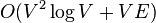 time. On unweighted graphs, calculating betweenness centrality takes
  time using Brandes' algorithm[5].
In calculating betweenness and closeness centralities of all vertices in a graph, it is assumed that graphs are undirected and connected with the allowance of loops and multiple edges. When specifically dealing with network graphs, oftentimes graphs are without loops or multiple edges to maintain simple relationships (where edges represent connections between two people or vertices). In this case, using Brandes' algorithm will divide final centrality scores by 2 to account for each shortest path being counted twice[5].
Closeness centrality
In w:topology and related areas in mathematics, closeness is one of the basic concepts in a topological space. Intuitively we say two sets are close if they are arbitrarily near to each other. The concept can be defined naturally in a w:metric space where a notion of distance between elements of the space is defined, but it can be generalized to topological spaces where we have no concrete way to measure distances.
In w:graph theory closeness is a centrality measure of a vertex within a graph. Vertices that are 'shallow' to other vertices (that is, those that tend to have short geodesic distances to other vertices with in the graph) have higher closeness. Closeness is preferred in w:network analysis to mean shortest-path length, as it gives higher values to more central vertices, and so is usually positively associated with other measures such as degree.
In the network theory, closeness is a sophisticated measure of centrality. It is defined as the mean geodesic distance (i.e., the shortest path) between a vertex v and all other vertices reachable from it:
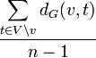
where  is the size of the network's 'connectivity component' V reachable from v.
Closeness can be regarded as a measure of how long it will take information to spread from a given vertex to other reachable vertices in the network[6].
is the size of the network's 'connectivity component' V reachable from v.
Closeness can be regarded as a measure of how long it will take information to spread from a given vertex to other reachable vertices in the network[6].
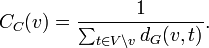
Some define closeness to be the reciprocal of this quantity, but either way the information communicated is the same (this time estimating the speed instead of the timespan). The closeness  for a vertex is the reciprocal of the sum of geodesic distances to all other vertices of V[7]:
Different methods and algorithms can be introduced to measure closeness, like the random-walk centrality introduced by Noh and Rieger (2003) that is a measure of the speed with which randomly walking messages reach a vertex from elsewhere in the network—a sort of random-walk version of closeness centrality[8].
The information centrality of Stephenson and Zelen (1989) is another closeness measure, which bears some similarity to that of Noh and Rieger. In essence it measures the harmonic mean length of paths ending at a vertex i, which is smaller if i has many short paths connecting it to other vertices[9].
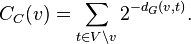
Dangalchev (2006), in order to measure the network vulnerability, modifies the definition for closeness so it can be used for disconnected graphs and the total closeness is easier to calculate[10]:
An extension to networks with disconnected components has been proposed by Opsahl (2010)[11].
Eigenvector centrality
Eigenvector centrality is a measure of the importance of a node in a network. It assigns relative scores to all nodes in the network based on the principle that connections to high-scoring nodes contribute more to the score of the node in question than equal connections to low-scoring nodes. w:Google's w:PageRank is a variant of the Eigenvector centrality measure.
Using the adjacency matrix to find eigenvector centrality
Let  denote the score of the
  node. Let
  be the w:adjacency matrix of the network. Hence
  if the node is adjacent to the
  node, and
  otherwise. More generally, the entries in A can be real numbers representing connection strengths, as in a w:stochastic matrix.
For the node, let the centrality score be proportional to the sum of the scores of all nodes which are connected to it. Hence
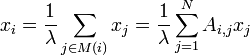
where  is the set of nodes that are connected to the node, N is the total number of nodes and
  is a constant. In vector notation this can be rewritten as
 , or as the w:eigenvector equation
In general, there will be many different w:eigenvalues for which an eigenvector solution exists. However, the additional requirement that all the entries in the eigenvector be positive implies (by the w:Perron–Frobenius theorem) that only the greatest eigenvalue results in the desired centrality measure.[12] The component of the related eigenvector then gives the centrality score of the node in the network. w:Power iteration is one of many w:eigenvalue algorithms that may be used to find this dominant eigenvector.
See also
Notes and references
- ↑ Centrality measures http://en.wikipedia.org/wiki/Centrality
- ↑ An introduction to centrality measures. http://sites.google.com/site/networkanalysisacourse/schedule/an-introduction-to-centrality-measures
- ↑ Opsahl, Tore; Agneessens, Filip; Skvoretz, John (2010). "Node centrality in weighted networks: Generalizing degree and shortest paths". Social Networks 32: 245. doi:10.1016/j.socnet.2010.03.006. http://toreopsahl.com/2010/04/21/article-node-centrality-in-weighted-networks-generalizing-degree-and-shortest-paths/.
- ↑ Template:Cite thesis
- 1 2 Ulrik Brandes (PDF). A faster algorithm for betweenness centrality. http://www.cs.ucc.ie/~rb4/resources/Brandes.pdf.
- ↑ Newman, MEJ, 2003, Arxiv preprint cond-mat/0309045.
- ↑ Sabidussi, G. (1966) The centrality index of a graph. Psychometrika 31, 581--603.
- ↑ J. D. Noh and H. Rieger, Phys. Rev. Lett. 92, 118701 (2004).
- ↑ Stephenson, K. A. and Zelen, M., 1989. Rethinking centrality: Methods and examples. Social Networks 11, 1–37.
- ↑ Dangalchev Ch., Residual Closeness in Networks, Phisica A 365, 556 (2006).
- ↑ Tore Opsahl. Closeness centrality in networks with disconnected components. http://toreopsahl.com/2010/03/20/closeness-centrality-in-networks-with-disconnected-components/.
- ↑ M. E. J. Newman (PDF). The mathematics of networks. http://www-personal.umich.edu/~mejn/papers/palgrave.pdf. Retrieved 2006-11-09.
Further reading
- Freeman, L. C. (1979). Centrality in social networks: Conceptual clarification. Social Networks, 1(3), 215-239.
- Sabidussi, G. (1966). The centrality index of a graph. Psychometrika, 31 (4), 581-603.
- Freeman, L. C. (1977) A set of measures of centrality based on betweenness. Sociometry 40, 35-41.
- Koschützki, D.; Lehmann, K. A.; Peeters, L.; Richter, S.; Tenfelde-Podehl, D. and Zlotowski, O. (2005) Centrality Indices. In Brandes, U. and Erlebach, T. (Eds.) Network Analysis: Methodological Foundations, pp. 16–61, LNCS 3418, Springer-Verlag.
- Bonacich, P.(1987) Power and Centrality: A Family of Measures, The American Journal of Sociology, 92 (5), pp 1170–1182
External links
- https://networkx.lanl.gov/trac/attachment/ticket/119/page_rank.py
- http://www.faculty.ucr.edu/~hanneman/nettext/C10_Centrality.html