Transportation Economics/Utility

< Transportation Economics

Utility is the economists representation of whatever consumers try to maximize. Consumers may want more of one thing and less of another. ...

Indifference Curves

Indifference curve

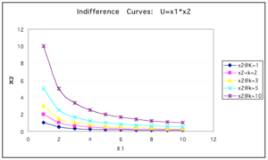
Demand depends on utility. Utility functions represent a way of assigning rankings to different bundles such that more preferred bundles are ranked higher than less preferred bundles. A utility function can be represented in a general way as:

$U=U(x_{1},x_{2}) = x_{1}x_{2} \,\!$

where $x_{1}$ and $x_{2}$ are goods (e.g. the net benefits resulting from a trip)

An indifference curve is the locus of commodity bundles over which a consumer is indifferent. If preferences satisfy the usual regularity conditions (discussed below), then there is a utility function $U(x_{1},x_{2})$ that represents these preferences. Points along the indifference curve represent iso-utility. The negative slope indicates the marginal rate of substitution (MRS):

$MRS=-\frac{\Delta x_{2}}{\Delta x_{1}} \,\!$

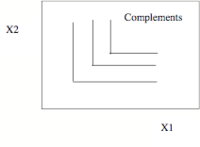
Substitutes and Complements

Substitute goods

Complements curve

Substitutes would be represented by :

$U(x_{1},x_{2}) = ax_{1}+bx_{2} \,\!$

where the slope of the indifference curve would be = -a/b.

In graphic terms substitutability is greater the more the indifference curves approach a straight line. Perfect substitutability is a straight line indifference curve (e.g. trips to work by mode A or mode B).

Complements are represented by:

$U(x_{1},x_{2}) = min(x_{1},x_{2}) \,\!$

The more complementary the more the indifference curves approach a right angle curve; perfect complementarity would have a right angle indifference curve (eg. left and right shoes, trips from home to work and work to home)

Trade Game

The trade game is a way of examining how economic trading of resources affects individual utility. Imagine the economy consists of the following resources (denoted by colored slips of paper)

White
Purple
Brown
Orange
Blue
Gray
Green
Yellow
Gold

The objective of the game is to maximize your gains in utility.

Define A Utility Function for Yourself

$U = f(\text{White, Purple, Brown, Orange, Blue, Gray, Green, Yellow, Gold})$

You are handed an assortment of resources

Measure your utility

Trade with others in the class (15 minutes) Record your trades.

At the end of the trading period measure your utility again. Compute your absolute and percentage increase.

Record scores on the board

Discuss

Is there a better way to allocate resources?

Preference Maximization

Graphical

Budget constraints

Budget curve moves outward

Slope of budget curve changes

Optimization of utility

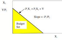
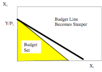
Utility maximization involves the choice of bundles under a resource constraint. For example, individuals select the amount of goods, services and transportation by comparing the utility increase with an increase in consumption against the utility loss associated with the giving up of resources (or equivalently forgoing the consumption which those resources command).

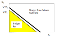
Often one price is taken to be 1, and one good is taken to be money. An income increase can be represented by the outward movement of the budget line.

An increase in the price of good $X_{1}$ can be represented by a change in the slope of the budget line (still anchored at one end).

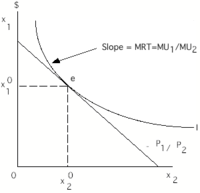
In graphic terms the process of optimization is accomplished by equating the rate at which an individual is willing to trade off one good for another to the rate at which the market allows him/her to trade them off. This can be represented in the following graph

The individual maximizes utility by moving down the budget constraint to that point at which the slope of the budget line ( $-P_1/P_2$ ) which is the rate of exchange dictated by the market is just equal to the rate at which the individual is willing to trade the two goods off. This is the slope of the indifference curve or the marginal rate of transformation (MRT). A point such as 'e' is an equilibrium point at which utility is being maximized.

Equilibrium is the tangency between the indifference curve/utility and the budget constraint.

Optimization

As an optimization problem, this can be written:

$\text{Maximize} U(X) \,\!$

subject to:

$px \le m \,\!$

$x$ is in $X$

where:

$p$ = price vector,
$x$ = goods vector,
$m$ = income

(Because of non-satiation, the constraint can be written as px=m.) This kind of problem can be solved with the use of the Lagrangian:

$\Lambda = U(X) - \lambda (px - m) \,\!$ where

$\lambda$ is the Lagrange multiplier

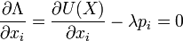
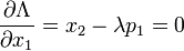
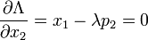
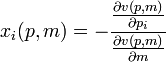
Take derivatives with respect to $x$ , and set the first order conditions to 0

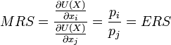
$\frac{\partial \Lambda}{\partial x_{i}}=\frac{\partial U(X)}{\partial x_{i}}-\lambda p_{i}=0 \,\!$

Divide to get the Marginal rate of substitution and Economic Rate of Substitution

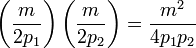
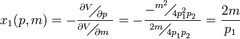
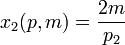
$MRS=\frac{\frac{\partial U(X)}{\partial x_{i}}}{\frac{\partial U(X)}{\partial x_{j}}}=\frac{p_{i}}{p_{j}}=ERS \,\!$

Example: Optimizing Utility

$\text{Max} U=x_{1}x_{2} \,\!$

$\text{s.t.} m=p_{1}x_{1}+p_{2}x_{2} \,\!$

$\Lambda=x_{1}x_{2}-\lambda (p_{1}x_{1}+p_{2}x_{2}-m) \,\!$

$\frac{\partial \Lambda}{\partial x_{1}}=x_{2}-\lambda p_{1}=0 \,\!$

$\frac{\partial \Lambda}{\partial x_{2}}=x_{1}-\lambda p_{2}=0 \,\!$

Solving

$\frac{x_{2}}{p_{1}}=\frac{x_{1}}{p_{2}} \,\!$

$p_{1}x_{1}\text{ }=\text{ }p_{2}x_{2} \,\!$

substituting into the budget constraint:

$m=2p_{1}x_{1} \,\!$

$x_{_{1}}^{*}=\frac{m}{2p_{1}} \,\!$

$x_{_{2}}^{*}=\frac{m}{2p_{2}} \,\!$

Demand, Expenditure, and Utility

Indirect Utility

The Marshallian Demand relates price and income to the demanded bundle. This is given as $x(p,m)$ . This function is homogenous of degree 0, so if we double both $p$ and $m$ , $x$ remains constant. We can develop an indirect utility function:

$v(p,m)=max U(X) \,\!$

subject to: $px=m \,\!$

where X that solves this is the demanded bundle

Example: Indirect Utility

$\left( \frac{m}{\text{2}p_{1}} \right)\left( \frac{m}{\text{2}p_{2}} \right)=\frac{m^{2}}{4p_{1}p_{2}} \,\!$

taking a monotonic transform:

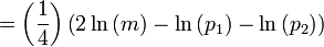
$=\left( \frac{1}{4} \right)\left( 2\ln \left( m \right)-\ln \left( p_{1} \right)-\ln \left( p_{2} \right) \right) \,\!$

which increases in income and decreases in price

where the $X$ that solves this is the demanded bundle

Properties

Properties of the indirect utility function $v(p,m)$

is non-increasing in $p$ , non-decreasing in $m$
homogenous of degree 0
quasiconvex in $p$
continuous at all $p >>0, m> 0$

Expenditure Function

The inverse of the indirect utility is the expenditure function $e(p,u) = \text{min} px \,\!$

subject to: $u(x) \ge u \,\!$

Properties of the expenditure function $e(p,u)$ :

is non-decreasing in $p$
homogenous of degree 1 in $p$
concave in $p$
continuous in $p$ for $p >>0$

Roy's Identity

The Hicksian Demand or compensated demand is denoted h(p,u).

$h_{i}(p,u)=\frac{\partial e(p,u)}{\partial p_{i}} \,\!$

vary price and income to keep consumer at fixed utility level vs. Marshallian demand. Roy's Identity allows going back and forth between observed demand and utility

$x_{i}(p,m)=-\frac{\frac{\partial v(p,m)}{\partial p_{i}}}{\frac{\partial v(p,m)}{\partial m}} \,\!$

Example (continued)

$x_{1}(p,m)=-\frac{{}^{\partial V}\!\!\diagup\!\!{}_{\partial p}\;}{{}^{\partial V}\!\!\diagup\!\!{}_{\partial m}\;}=-\frac{-{}^{m^{2}}\!\!\diagup\!\!{}_{4p_{1}^{2}p_{2}^{{}}}\;}{{}^{2m}\!\!\diagup\!\!{}_{4p_{1}^{{}}p_{2}^{{}}}\;}=\frac{2m}{p_{1}} \,\!$

$x_{2}(p,m)=\frac{2m}{p_{2}} \,\!$

Equivalencies

$e(p,v(p,m)) = m \,\!$ the minimum expenditure to reach $v(p,m)$ is $m$

$v(p,e(p,u)) = u \,\!$ the maximum utility from income $e(p,u)$ is $u$

$x_{i} (p,m) = h_{i}(p,v(p,m)) \,\!$ Marshallian demand at $m$ is Hicksian demand at $v(p,m)$

$h_{i} (p,u) = x_{i} (p,e(p,u)) \,\!$ Hicksian demand at $u$ is Marshallian demand at $e(p,u)$

Measuring Welfare

Money Metric Indirect Utility Function

The Money Metric Indirect Utility Function tells how much money at price p is required to be as well off as at price level q and income m. Define it as

$\mu(p;q,m)=e(p,v(q,m)) \,\!$

Equivalent Variation

$EV = \mu(p^0;p^1,m^1) - \mu(p^0;p^0,m^0) \,\!$

note 1 indicates after, 0 indicates before

Current prices are the base, what income change will give equivalent utility

Compensating Variation

$CV = \mu(p^1;p^1,m^1) - \mu(p^1;p^0,m^0) \,\!$ New prices are the base, what income change will compensate for price change

Consumer's Surplus

Utility and Consumer's Surplus

$\Delta CS=\int\limits_{p^{0}}^{p^{1}}{x(t)dt} \,\!$

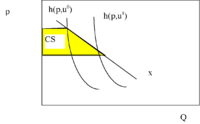
Generally

$EV \ge CS \ge CV \,\!$

When utility is quasilinear ( $U=U(X1)+X0)\,\!$ , then:

$EV = CS = CV\,\!$

Arrow's Impossibility Theorem

Arrow's Impossibility Theorem An illustration of the problem of aggregation of social welfare functions:

Three individuals each have well-behaved preferences. However, aggregating the three does not produce a well behaved preference function:

Person A prefers red to blue and blue to green
Person B prefers green to red and red to blue
Person C prefers blue to green and green to red.

Aggregating, transitivity is violated.

Two people prefer red to blue
Two people prefer blue to green, and
Two people prefer green to red.

What does society want?

Preferences

Consumption Bundles

Define a consumption set X, e.g. {house, car, computer},

'x', 'y', 'z', are bundles of goods, such as x{house,car}, y{car, computer}, z{house, computer}.

Goods are not consumed for themselves but for their attributes relative to other goods

We want to find preferences that order the bundles. Utility is ordinal, so we only care about which is greater, not by how much.

Conditions

There are several Conditions on preferences to produce a continuous (well-behaved) utility function.

Completeness: Either $x \underline \succ y$ (Read x is preferred to y) or $y \underline \succ x$ or both
Reflexive: $x\underline \succ x$
Transitive: if $x\underline \succ y$ and $y\underline \succ z$ then $x\underline \succ z$ (This poses a problem for social welfare functions)
Monotonicity: If $x \ge y$ then $x \underline \succ y$
Local Non-satiation: More is better than less
Convexity: if $x\underline \succ y$ and $y\underline \succ z$ then $tx+(1-t)y \underline \succ z$
Continuity: small changes in input beget small changes in output. The preference relation $\underline \succ$ in X is continuous if it is preserved under the limit operation