Signal Processing/Image Editing

< Signal Processing

As an image is a type of 2-D signal; instead of just time-amplitude pairs that correspond to a voice transmission, consider "time in the X domain"-"time in the Y domain"-amplitude pairs. That is, an X coordinate, a Y coordinate and an amplitude. This will give you a monochromatic image. As such, signal processing tools can be used in editing images.

Singular Value Decomposition

The Singular Value Decomposition is a matrix decomposition (another way to say factorization).

M = U\Sigma V^*

where

U is an m×m unitary matrix over.
Σ is an m×n diagonal matrix with nonnegative real numbers s_{n,n} on the diagonal where

s_{1,1}> s_{2,2} > \ldots s_{n,n}

V*, an n×n unitary matrix. V* is the conjugate transpose (take the complex conjugate of all entries, and then perform a transpose operation on the matrix) of V.

The diagonal entries Σ_i,i of Σ are known as the singular values of M.

Image Compression

The nature of the singular values Σ is such that for a certain k,

s_{1,1}> s_{2,2} >> s_{k,k} > \ldots s_{n,n}

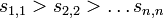
In order to transmit a 10x10 monochromatic image with 2 values ("on" or "off") it would require a matrix that has 10x10 = 100 entries. Consider the following image.

This image can be represented by the following matrix.

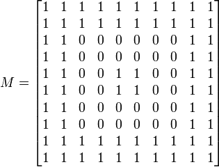
M = \begin{bmatrix} 1 & 1 & 1 & 1 & 1 & 1 & 1 & 1 & 1 & 1\\ 1 & 1 & 1 & 1 & 1 & 1 & 1 & 1 & 1 & 1\\ 1 & 1 & 0 & 0 & 0 & 0 & 0 & 0 & 1 & 1\\ 1 & 1 & 0 & 0 & 0 & 0 & 0 & 0 & 1 & 1\\ 1 & 1 & 0 & 0 & 1 & 1 & 0 & 0 & 1 & 1\\ 1 & 1 & 0 & 0 & 1 & 1 & 0 & 0 & 1 & 1\\ 1 & 1 & 0 & 0 & 0 & 0 & 0 & 0 & 1 & 1\\ 1 & 1 & 0 & 0 & 0 & 0 & 0 & 0 & 1 & 1\\ 1 & 1 & 1 & 1 & 1 & 1 & 1 & 1 & 1 & 1\\ 1 & 1 & 1 & 1 & 1 & 1 & 1 & 1 & 1 & 1\end{bmatrix}

The singular value decomposition of which is

M = U\Sigma V^*,

Where

\Sigma = \begin{bmatrix} 7.557 & 0 & 0 & 0 & 0 & 0 & 0 & 0 & 0 & 0\\ 0 & 2.979 & 0 & 0 & 0 & 0 & 0 & 0 & 0 & 0\\ 0 & 0 & 1.422 & 0 & 0 & 0 & 0 & 0 & 0 & 0\\ 0 & 0 & 0 & 0 & 0 & 0 & 0 & 0 & 0 & 0\\ 0 & 0 & 0 & 0 & 0 & 0 & 0 & 0 & 0 & 0\\ 0 & 0 & 0 & 0 & 0 & 0 & 0 & 0 & 0 & 0\\ 0 & 0 & 0 & 0 & 0 & 0 & 0 & 0 & 0 & 0\\ 0 & 0 & 0 & 0 & 0 & 0 & 0 & 0 & 0 & 0\\ 0 & 0 & 0 & 0 & 0 & 0 & 0 & 0 & 0 & 0\\ 0 & 0 & 0 & 0 & 0 & 0 & 0 & 0 & 0 & 0\end{bmatrix}

Using the matrix

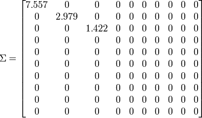
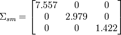
\Sigma_{sm} = \begin{bmatrix} 7.557 & 0 & 0\\ 0 & 2.979 & 0\\ 0 & 0 & 1.422\end{bmatrix}

And corresponding "truncated" versions of U and V* (Use only the first three columns of U and the first three columns of V*), we can find that

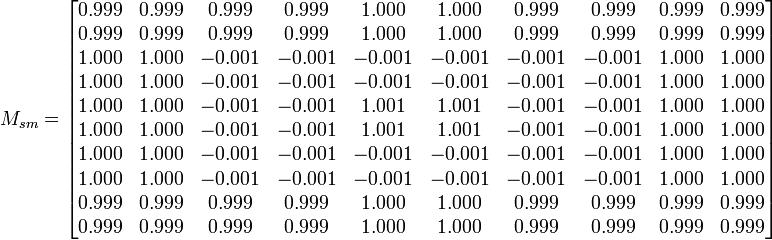
M_{sm}= \begin{bmatrix} 0.999 & 0.999 & 0.999 & 0.999 & 1.000 & 1.000 & 0.999 & 0.999 & 0.999 & 0.999\\ 0.999 & 0.999 & 0.999 & 0.999 & 1.000 & 1.000 & 0.999 & 0.999 & 0.999 & 0.999\\ 1.000 & 1.000 &-0.001 &-0.001 &-0.001 &-0.001 &-0.001 &-0.001 & 1.000 & 1.000\\ 1.000 & 1.000 &-0.001 &-0.001 &-0.001 &-0.001 &-0.001 &-0.001 & 1.000 & 1.000\\ 1.000 & 1.000 &-0.001 &-0.001 & 1.001 & 1.001 &-0.001 &-0.001 & 1.000 & 1.000\\ 1.000 & 1.000 &-0.001 &-0.001 & 1.001 & 1.001 &-0.001 &-0.001 & 1.000 & 1.000\\ 1.000 & 1.000 &-0.001 &-0.001 &-0.001 &-0.001 &-0.001 &-0.001 & 1.000 & 1.000\\ 1.000 & 1.000 &-0.001 &-0.001 &-0.001 &-0.001 &-0.001 &-0.001 & 1.000 & 1.000\\ 0.999 & 0.999 & 0.999 & 0.999 & 1.000 & 1.000 & 0.999 & 0.999 & 0.999 & 0.999\\ 0.999 & 0.999 & 0.999 & 0.999 & 1.000 & 1.000 & 0.999 & 0.999 & 0.999 & 0.999\end{bmatrix}

A cursory examination of the previous matrix will show that M_{sm} is approximately equal to M. Note that the truncated version of U and V* use 3*10 numbers each. The total number of values needed for this type of storage is 2*30+3 = 63. Which means data usage is reduced by nearly half.

This article is issued from Wikibooks. The text is licensed under Creative Commons - Attribution - Sharealike. Additional terms may apply for the media files.