Numerical Methods/Numerical Integration
< Numerical MethodsOften, we need to find the integral of a function that may be difficult to integrate analytically (ie, as a definite integral) or impossible (the function only existing as a table of values).
Some methods of approximating said integral are listed below.
Trapezoidal Rule
Consider some function, possibly unknown,  , with known values over the interval [a,b] at n+1 evenly spaced points xi of spacing
 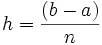 ,
,  and
and  .
.
Further, denote the function value at the ith mesh point as  .
.
Using the notion of integration as "finding the area under the function curve", we can denote the integral over the ith segment of the interval, from  to
to  as:
as:
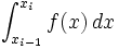 = (1)
= (1)
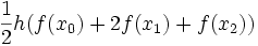
Since we may not know the antiderivative of , we must approximate it. Such approximation in the Trapezoidal Rule, unsurprisingly, involves approximating (1) with a trapezoid of width h, left height  , right height . Thus,
(1) 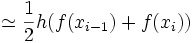 = (2)
= (2)
(2) gives us an approximation to the area under one interval of the curve, and must be repeated to cover the entire interval.
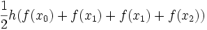
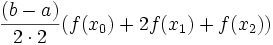
For the case where n = 2,
 = (3)
= (3)
Collecting like terms on the right hand side of (3) gives us:
or
Now, substituting in for h and cleaning up,
To motivate the general version of the trapezoidal rule, now consider n = 4,

Following a similar process as for the case when n=2, we obtain
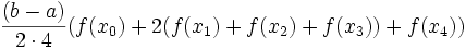
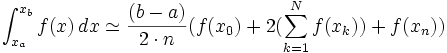
Proceeding to the general case where n = N,
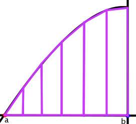 This is an example of what the trapezoidal rule would represent graphicly, here
 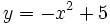 .
.
Example
Approximate  to within 5%.
First, since the function can be exactly integrated, let us do so, to provide a check on our answer.
![\int_{0}^{1} x^3\, dx = \left [{x^4 \over 4}\right ]_0^1 = {1 \over 4} = 0.25](../I/m/fef2592571880e2ef0d2fae15bd9a683.png) = (4)
= (4)
We will start with an interval size of 1, only considering the end points.


(4) 
Relative error = 
Hmm, a little high for our purposes. So, we halve the interval size to 0.5 and add to the list
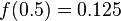
(4) 
Relative error = 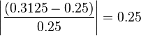
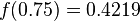
Still above 0.01, but vastly improved from the initial step. We continue in the same fashion, calculating  and
and  , rounding off to four decimal places.
(4) 
Relative error = 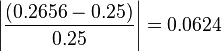
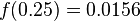
We are well on our way. Continuing, with interval size 0.125 and rounding as before,
(4) 
Relative error = 
Since our relative error is less than 5%, we stop.
Error Analysis
Let y=f(x) be continuous,well-behaved and have continuous derivatives in [x0,xn]. We expand y in a Taylor series about x=x0,thus-
![\int_{x_0}^{x_1}y\, dx=\int_{x_0}^{x_1}[y_0+(x-x_0)y'_0+(x-x_0)^2y''_0/2!+......]\,dx](../I/m/a4132836a96f3497868e338c7842f62b.png)
Simpson's Rule
Consider some function  possibily unknown with known values over the interval [a,b] at n+1 evently spaced points then it defined as

where and and .
Example
Evaluate 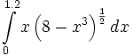 by taking
  (
( must be even)
Solution: Here 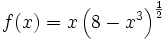
Since  &
&  so
so 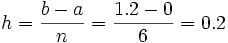
Now when  then
then 
And since  , therefore for
  ,
,  ,
,  ,
,  ,
,  ,
,  the corresponding values are
  ,
,  ,
,  ,
,  ,
,  ,
, 
Incomplete ... Completed soon
Simpson's 3/8
The numerical integration technique known as "Simpson's 3/8 rule" is credited to the mathematician Thomas Simpson (1710-1761) of Leicestershire, England. His also worked in the areas of numerical interpolation and probability theory.
Theorem (Simpson's 3/8 Rule) Consider over , where , , and . Simpson's 3/8 rule is
.
This is an numerical approximation to the integral of over and we have the expression
.
The remainder term for Simpson's 3/8 rule is , where lies somewhere between , and have the equality
.
Proof Simpson's 3/8 Rule Simpson's 3/8 Rule
Composite Simpson's 3/8 Rule
Our next method of finding the area under a curve is by approximating that curve with a series of cubic segments that lie above the intervals . When several cubics are used, we call it the composite Simpson's 3/8 rule.
Theorem (Composite Simpson's 3/8 Rule) Consider over . Suppose that the interval is subdivided into subintervals of equal width by using the equally spaced sample points for . The composite Simpson's 3/8 rule for subintervals is
.
This is an numerical approximation to the integral of over and we write
.
Proof Simpson's 3/8 Rule Simpson's 3/8 Rule
Remainder term for the Composite Simpson's 3/8 Rule
Corollary (Simpson's 3/8 Rule: Remainder term) Suppose that is subdivided into subintervals of width . The composite Simpson's 3/8 rule
.
is an numerical approximation to the integral, and
.
Furthermore, if , then there exists a value with so that the error term has the form
.
This is expressed using the "big " notation .
Remark. When the step size is reduced by a factor of the remainder term should be reduced by approximately .
Algorithm Composite Simpson's 3/8 Rule. To approximate the integral
,
by sampling at the equally spaced sample points for , where . Notice that and .
Animations (Simpson's 3/8 Rule Simpson's 3/8 Rule). Internet hyperlinks to animations.
Computer Programs Simpson's 3/8 Rule Simpson's 3/8 Rule
Mathematica Subroutine (Simpson's 3/8 Rule). Object oriented programming.
Example 1. Numerically approximate the integral by using Simpson's 3/8 rule with m = 1, 2, 4.
Solution 1.
Example 2. Numerically approximate the integral by using Simpson's 3/8 rule with m = 10, 20, 40, 80, and 160. Solution 2.
Example 3. Find the analytic value of the integral (i.e. find the "true value"). Solution 3.
Example 4. Use the "true value" in example 3 and find the error for the Simpson' 3/8 rule approximations in example 2. Solution 4.
Example 5. When the step size is reduced by a factor of the error term should be reduced by approximately . Explore this phenomenon. Solution 5.
Example 6. Numerically approximate the integral by using Simpson's 3/8 rule with m = 1, 2, 4. Solution 6.
Example 7. Numerically approximate the integral by using Simpson's 3/8 rule with m = 10, 20, 40, 80, and 160. Solution 7.
Example 8. Find the analytic value of the integral (i.e. find the "true value"). Solution 8.
Example 9. Use the "true value" in example 8 and find the error for the Simpson's 3/8 rule approximations in example 7. Solution 9.
Example 10. When the step size is reduced by a factor of the error term should be reduced by approximately . Explore this phenomenon. Solution 10.
Various Scenarios and Animations for Simpson's 3/8 Rule.
Example 11. Let over . Use Simpson's 3/8 rule to approximate the value of the integral. Solution 11.
Animations (Simpson's 3/8 Rule Simpson's 3/8 Rule). Internet hyperlinks to animations.
Research Experience for Undergraduates
Simpson's Rule for Numerical Integration Simpson's Rule for Numerical Integration Internet hyperlinks to web sites and a bibliography of articles.
Headline text
Error Analysis
References
Eric W. Weisstein. "Trapezoidal Rule." From MathWorld--A Wolfram Web Resource. http://mathworld.wolfram.com/TrapezoidalRule.html
Main Page - Mathematics bookshelf - Numerical Methods