Numerical Methods/Interpolation
< Numerical MethodsInterpolation
Polynomial Interpolation
Interpolation is way of extending discrete data points to a function. If the given data points are in  then polynomial interpolation is common. The main idea behind polynomial interpolation is that given n+1 discrete data points there exits a unique polynomial of order n that fits those data points. A polynomial of lower order is not generally possible and a polynomial of higher order is not unique. If the polynomial
  is defined as

then the unknown coefficients can be solved for with the system
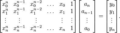
where  are the given data points. The matrix in the system is known as the Vandermonde matrix. Assume all of the data points are distinct the Vandermonde matrix is nonsingular and therefore the system can be uniquely solved.
If the number of data points being interpolated on becomes large the degree of the polynomial will become large which may result in oscillations between data points and an increase in error. For large numbers of data points alternative methods are suggested.
Radial Basis Functions
A common problem in science and engineering is that of multivariate
interpolation of a function f whose values are known only on a finite set of points. Therefore let
 be an open bounded domain. Given a set of distinct points X
and real numbers, the task is to construct a function
be an open bounded domain. Given a set of distinct points X
and real numbers, the task is to construct a function
 that satisfies the interpolation conditions

In the last decades, the approach of radial basis function interpolation
became increasingly popular for problems in which the points in X
are irregularly distributed in space. In its basic form, radial basis
function interpolation chooses a fixed function
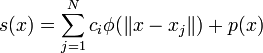
 and defines an interpolant by
 where the coefficients
  are real numbers, for
 one chooses usually the euclidian norm, and
is a radial basis function.
one chooses usually the euclidian norm, and
is a radial basis function.
We see that the approximating function
s is a linear combination of radially symmetric functions,
each centered on a definite point  . The points
often called the centers or collocation points of the RBF interpolant.
This approach goes back to Hardy,
who used as early as 1971 the multi-quadric RBF to reconstruct geographical
surfaces from a set of scattered measurements.
Note also that the centers
. The points
often called the centers or collocation points of the RBF interpolant.
This approach goes back to Hardy,
who used as early as 1971 the multi-quadric RBF to reconstruct geographical
surfaces from a set of scattered measurements.
Note also that the centers  can be located at arbitrary
points in the domain, and do not require a grid. For certain RBF exponential
convergence has been shown. Radial basis functions were successfully
applied to problems as diverse as computer graphics, neural networks,
for the solution of differential equations via collocation methods
and many other problems.
can be located at arbitrary
points in the domain, and do not require a grid. For certain RBF exponential
convergence has been shown. Radial basis functions were successfully
applied to problems as diverse as computer graphics, neural networks,
for the solution of differential equations via collocation methods
and many other problems.
Other popular choices for comprise the Gaussian function and
the so called thin plate splines, invented by Duchon in the 1970s. Thin plate splines result from the
solution of a variational problem. The advantage of the thin plate
splines is that their conditioning is invariant under scalings. Another
class of functions are Wendland's compactly supported RBF, which are
relevant because they lead to a sparse interpolation matrix, and thus
the resulting linear system can be solved efficiently. However, the
conditioning of the problem gets worse with the number of centers.
When interpolating with RBF of global support, the matrix A
usually becomes ill-conditioned with an increasing number of centers.
Gaussians, multi-quadrics and inverse multi-quadrics are infinitely smooth and involve a scale- or shape parameter,  > 0.
\ref{fig:var-eps2} for the Gaussian RBF with different values of
. Decreasing tends to flatten the basis function.
For a given function, the quality of approximation may strongly depend on this
parameter. In particular, increasing
has the effect of better conditioning (the separation distance
> 0.
\ref{fig:var-eps2} for the Gaussian RBF with different values of
. Decreasing tends to flatten the basis function.
For a given function, the quality of approximation may strongly depend on this
parameter. In particular, increasing
has the effect of better conditioning (the separation distance 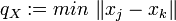 of the scaled points increases).
Solving the interpolation problem results in the linear system of equations

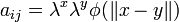
with
 . Because only the distance between
the points appears in A, the effort to solve the system is
independent of the spatial dimension, which becomes important especially
when interpolating in higher dimensions. Franke
posed in 1982 the question whether the matrix A is nonsingular
and thus a unique interpolant is guaranteed to exist for any choice
of f. A few years later, this conjecture was proven true for
a number of useful RBF independently by results of Micchelli
and Madych and Nelson. The only requirement is
that there are at least two centers and that all centers are distinct.
An exception are the thin plate splines, for which the matrix A
can be singular for nontrivial distributions of points. For example, if the points
. Because only the distance between
the points appears in A, the effort to solve the system is
independent of the spatial dimension, which becomes important especially
when interpolating in higher dimensions. Franke
posed in 1982 the question whether the matrix A is nonsingular
and thus a unique interpolant is guaranteed to exist for any choice
of f. A few years later, this conjecture was proven true for
a number of useful RBF independently by results of Micchelli
and Madych and Nelson. The only requirement is
that there are at least two centers and that all centers are distinct.
An exception are the thin plate splines, for which the matrix A
can be singular for nontrivial distributions of points. For example, if the points
 are distributed on the unit sphere around the center
 , then the first row and column consists
of zeros. A remedy for this problem is to add to the interpolant a
polynomial p of degree
, then the first row and column consists
of zeros. A remedy for this problem is to add to the interpolant a
polynomial p of degree  , so that the interpolant becomes
and to require that the node points are unisolvent (for  ), that means every polynomial
 is determined by its values on X.
denotes the space of all polynomials in n variables up to degree m
and the
is determined by its values on X.
denotes the space of all polynomials in n variables up to degree m
and the  are the standard basis polynomials for this space.
A point set is unisolvent for
are the standard basis polynomials for this space.
A point set is unisolvent for  if all points are distinct,
unisolvent for
if all points are distinct,
unisolvent for  of not all points are arranged on one
line.
of not all points are arranged on one
line.
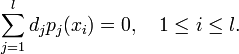
The interpolation conditions are now
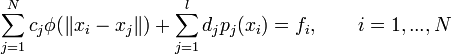
Because the interpolation conditions result in N equations
in N + l unknowns, the system is under-determined. Therefore,
extra side conditions are imposed, which represent the property of
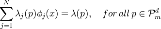
polynomial reproduction. This
means that if the data comes from a polynomial  ,
i.e.
,
i.e.  , then, the interpolant s must coincide with p. These conditions
amount to
, then, the interpolant s must coincide with p. These conditions
amount to
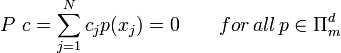
To find c and d, we need to solve the linear systems

where  and A is defined as above. The
equations may be summarized as
and A is defined as above. The
equations may be summarized as
The system has a unique solution, if the function belongs
to the following class of functions.
Definition A continuous function
 is said to be conditionally
positive definite of order m, shortly
is said to be conditionally
positive definite of order m, shortly  if for
every set
if for
every set 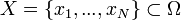 of distinct points
and for every set of complex values
of distinct points
and for every set of complex values  for which
the quadratic form
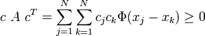
is positive. If, additionally  implies
  , then is said to be strictly
CPD of order m. For
, then is said to be strictly
CPD of order m. For  ,
,  is said to be positive
definite.
is said to be positive
definite.
A radial basis function  is called conditionally
positive definite if the corresponding multivariate function
is conditionally positive definite.
is called conditionally
positive definite if the corresponding multivariate function
is conditionally positive definite.
If a function is positive definite, then also the corresponding interpolation matrix is positive definite. TPS and MQ are conditionally positive definite functions, Gau, IMQ and Wen are positive definite functions.
Beside the proof of the problem to be well posed, a proof of the convergence is necessary. However, the convergence is guaranteed for most RBF only for global interpolation on infinite square grids. For the thin plate splines, also convergence proofs for local interpolation are known.
The Generalized Hermite Interpolation Problem
The interpolation problem can also be expressed in terms of
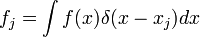
point evaluations i.e. applications of the Dirac delta functionals
acting on the function f. If  is a vector space
then the Dirac delta functional
is a vector space
then the Dirac delta functional  corresponding to x is defined by

The data is generated via
As before, let  be the centers. More generally,
the data can be generated by any set of linear functionals
be the centers. More generally,
the data can be generated by any set of linear functionals  acting on some function f. The distributions need to be independent
in order to avoid redundant data. The
acting on some function f. The distributions need to be independent
in order to avoid redundant data. The  are not restricted
to point evaluations, but can be arbitrary linear functionals including
differentiations and difference operators. This problem includes Hermite
functions and
are not restricted
to point evaluations, but can be arbitrary linear functionals including
differentiations and difference operators. This problem includes Hermite
functions and  the set of all distributions of compact
support. To a distribution
the set of all distributions of compact
support. To a distribution  corresponds a
linear functional, which is acting on
corresponds a
linear functional, which is acting on  via the convolution
of distributions. It can be written as
via the convolution
of distributions. It can be written as

Now, the task is to interpolate given the data, 
such that  satisfies

Here, the interpolant is of the form
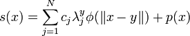
where, the  's are suitable real coefficients, and
  indicates that
  is acting on the viewed as a function
of the argument |y.
is acting on the viewed as a function
of the argument |y.
The entries of the interpolation matrix  in \ref{eq:rbf-lgs}
are now given by
in \ref{eq:rbf-lgs}
are now given by
If the number of linear functionals equals the number of centers and
if belongs to the class of conditionally positive definite
functions, then a unique solution does exist.