Maxima
This book shows how to use Maxima.
weaknesses of CAS/math software
- the limit of a discontinuous function at the point of discontinuity[1]
- branch cuts[2]
- zero-recognition
- keeping track of domains of validity
How to use ?
Ways to do it :
- online , wothout installation
- offline = after installation
Dependencies
- gnuplot,
- tex
- texinfo
- texi2html
- texlive-latex-recommended
- GNU autotools
- automake 1.9
- autoconf2.13
- tk 8.4.
- lisp
- sbcl
- libgmp3-dev
- libreadline5-dev
- libncurses5-dev
- sharutils
- libxmu-dev
- libxaw7-dev
- wxWidgets library for wxMaxima
- libwxgtk3.0-dev
- libwxbase3.0-dev
- compiler is GNU g++ for wxWidgets library
- build-essential
- imagemagick
- ibus-gtk
- ibus-gtk3
How to install ?
- Download and install ready made Maxima deb packages
- from Ubuntu repositories ( old versions )
- from other sites[3]
- Compile your own maxima package[4][5]
- compile maxima from sources ( without creating deb packages )
Now the best is a git method
from Ubuntu repositories
You can make use of :
- Synaptic ( Graphical package manager)
- apt-get.
In second case write in command line:[6]
sudo apt-get install maxima
This method can get old version which gets some trouble, like
loadfile: failed to load /usr/share/maxima/5.37.2/share/draw/draw.lisp
Uninstall such Maxima version
sudo apt-get remove maxima
from PPA
wxmaxima
From repositiories[7] by Istvan Balhota
sudo add-apt-repository ppa:blahota/wxmaxima
sudo apt-get update
sudo apt-get install wxmaxima
From sources
Before compilation, you should have all dependent packages
CSV
cd maxima
./bootstrap    # only if you downloaded the source code from cvs
./configure --enable-clisp   # or:   --enable-sbcl
make
make check
sudo make install
make clean
This procedure does not create a deb package.
using git
maxima/xmaxima
If you have git and SBCL then : [8]
  git clone git://git.code.sf.net/p/maxima/code maxima
  cd maxima
  ./bootstrap
  ./configure --with-sbcl
  make
Now one can run it from inside the source directory.
cd maxima
./maxima-local
The result :
Maxima branch_5_30_base_104_ged70fb2_dirty http://maxima.sourceforge.net
using Lisp SBCL 1.0.45.0.debian
Distributed under the GNU Public License. See the file COPYING.
Dedicated to the memory of William Schelter.
The function bug_report() provides bug reporting information.
(%i1)
Xmaxima can also be run :
cd ~/maxima
./xmaxima-local
or bash file :
#!/bin/bash

# save as a  in your home directory
# chmod +x m
# ./m

cd maxima
./xmaxima-local
wxMaxima is not present now.
Where is Maxima after standard ( as above) installation ?
locate maxima-local
example result :
 ~/Pobrane/maxima-5.38.1/maxima-local.in
 ~/Pobrane/maxima-5.38.1/xmaxima-local.in
 ~/maxima/maxima-local
 ~/maxima/maxima-local.in
 ~/maxima/xmaxima-local
 ~/maxima/xmaxima-local.in
 ~/maxima/interfaces/xmaxima/Tkmaxima/maxima-local.tcl
Note that it is a different directory then after apt-get installation. One can have 2 ( or more ) versions of Maxima on the disk )
wxmaxima
git clone https://github.com/andrejv/wxmaxima
problems
- Open a terminal
- type : sudo apt-get install gdb
- after gdb is installed type : gdb wxmaxima
- run and wait until it crashes
- and type : backtrace
Operators
"=" means syntactic equality. Check : is(equal(a,b))
Directories
Start Maxima and type the command:[9]
maxima_userdir;
this will tell you the directory that is being used as your user directory.
Numbers
Number types
binary numbers
(%i1) ibase;
(%o1) 10
(%i2) obase;
(%o2) 10
(%i3) ibase:2;
(%o3) 2
(%i4) x=1001110;
(%o4) x=78
Complex numbers
Argument
Principial value of argument of complex number in turns carg produces results in the range (-pi, pi] . It can be mapped to [0, 2*pi) by adding 2*pi to the negative values
carg_t(z):=
 block(
 [t],
 t:carg(z)/(2*%pi),  /* now in turns */
 if t<0 then t:t+1, /* map from (-1/2,1/2] to [0, 1) */
 return(t)
)$
On can order list of complex points according to it's argument :
l2_ordered: sort(l2, lambda([z1,z2], is(carg(z1) < carg(z2))))$
Predicate functions
(%i1) is(0=0.0);
(%o1) false
Compare :
(%i1) a:0.0$
(%i2)is(equal(a,0));
(%o2) true
List of predicate functions ( see p at the end ) :
- abasep
- alphacharp
- alphanumericp
- atom
- bfloatp
- blockmatrixp
- cequal
- cequalignore
- cgreaterp
- cgreaterpignore
- charp
- clessp
- clesspignore
- constantp
- constituent
- diagmatrixp
- digitcharp
- disjointp
- elementp
- emptyp
- evenp
- featurep
- floatnump
- if
- integerp
- intervalp
- is
- lcharp
- listp
- listp
- lowercasep
- mapatom
- matrixp
- matrixp
- maybe
- member
- nonnegintegerp
- nonscalarp
- numberp
- oddp
- operatorp
- ordergreatp
- orderlessp
- picture_equalp
- picturep
- poly_depends_p
- poly_grobner_subsetp
- polynomialp
- prederror
- primep
- ratnump
- ratp
- scalarp
- sequal
- sequalignore
- setequalp
- setp
- stringp
- subsetp
- subvarp
- symbolp
- symmetricp
- taylorp
- unknown
- uppercasep
- zeroequiv
- zeromatrixp
- zn_primroot_p
Number Theory
There are functions and operators useful with integer numbers
Elementary number theory
In Maxima there are some elementary functions like the factorial n! and the double factorial n!! defined as where is the greatest integer less than or equal to


Divisibility
Some of the most important functions for integer numbers have to do with divisibility:
gcd, ifactor, mod, divisors...
all of them well documented in help. you can view it with the '?' command.
Function ifactors takes positive integer and returns a list of pairs : prime factor and its exponent. For example :
a:ifactors(8);
[[2,3]]
It means that :

Other Functions
Continuus fractions :
(%i6) cfdisrep([1,1,1,1]);
(%o6) 1+1/(1+1/(1+1/1))
(%i7) float(%), numer;
(%o7) 1.666666666666667
Functions
For mathematical functions use always
define()
instead of
:=
There is only one small difference between them:
"The function definition operator. f(x_1, ..., x_n) := expr defines a function named f with arguments x_1, …, x_n and function body expr. := never evaluates the function body (unless explicitly evaluated by quote-quote )."
"Defines a function named f with arguments x_1, …, x_n and function body expr. define always evaluates its second argument (unless explicitly quoted). "[10]
Debugging
trace
In Maxima :
:lisp (setf *debugger-hook* nil)
Data structures
"Maxima's current array/matrix semantics are a mess, I must say, with at least four different kinds of object (hasharrays, explicit lists, explicit matrices, Lisp arrays) supporting subscripting with varying semantics. " [11]
"Maxima's concept of arrays, lists, and matrices is pretty confused, since various ideas have accreted in the many years of the project... Yes, this is a mess. Sorry about that. These are all interesting ideas, but there is no unifying framework. " [12]
Array
Maxima has two array types :[13]
- Undeclared arrays ( implemented as Lisp hash tables )
- Declared arrays ( implemented as Lisp arrays )
- created by the array function
- created by the make_array function.
Category: Arrays :
- array
- arrayapply
- arrayinfo
- arraymake
- arrays - global variable
- fillarray
- listarray
- make_array
- rearray
- remarray
- subvar
- use_fast_arrays
See also :
- array functions defined by := and define.
Undeclared array
Assignment creates an undeclared array.
(%i1) c[99] : 789;
(%o1)                          789
(%i2) c[99];
(%o2)                          789
(%i3) c;
(%o3)                           c
(%i4) arrayinfo (c);
(%o4)                   [hashed, 1, [99]]
(%i5) listarray (c);
(%o5)                         [789]
"If the user assigns to a subscripted variable before declaring the corresponding array, an undeclared array is created. Undeclared arrays, otherwise known as hashed arrays (because hash coding is done on the subscripts), are more general than declared arrays. The user does not declare their maximum size, and they grow dynamically by hashing as more elements are assigned values. The subscripts of undeclared arrays need not even be numbers. However, unless an array is rather sparse, it is probably more efficient to declare it when possible than to leave it undeclared. " ( from Maxima CAS doc)
"created if one does :
b[x+1]:y^2
(and b is not already an array, a list, or a matrix - if it were one of these an error would be caused since x+1 would not be a valid subscript for an art-q array, a list or a matrix).
Its indices (also known as keys) may be any object. It only takes one key at a time (b[x+1,u]:y would ignore the u). Referencing is done by b[x+1] ==> y^2. Of course the key may be a list, e.g.
b[[x+1,u]]:y
would be valid. "( from Maxima CAS doc)
Declared array
- declare array ( give a name and allocate memmory)
- fill array
- process array
array function
Function: array (name, type, dim_1, …, dim_n)
Creates an n-dimensional array. Here :
- type can be fixnum for integers of limited size or flonum for floating-point numbers
- n may be less than or equal to 5. The subscripts for the i'th dimension are the integers running from 0 to dim_i.
(%i5) array(A,2,2);
(%o5)                                  A
(%i8) arrayinfo(A);
(%o8)                      [declared, 2, [2,2]]
Because subscripts of array A elements are goes from 0 to dim so array A has :
( dim_1 + 1) * (dim_2 + 1) = 3*3 = 9
elements.
The array function can be used to transform an undeclared array into a declared array.
arraymake function
Function: arraymake (A, [i_1, …, i_n])
The result is an unevaluated array reference.
(%i12) arraymake(A,[3,3,3]);
(%o12)                    array_make(3, 3, 3)
                                           3, 3, 3
(%i13) arrayinfo(A);
       arrayinfo: A is not an array.
Function: make_array
Function: make_array (type, dim_1, …, dim_n)
Creates and returns a Lisp array.
Type may be :
- any
- flonum
- fixnum
- hashed
- functional.
There are n indices, and the i'th index runs from 0 to dim_i - 1.
The advantage of make_array over array is that the return value doesn't have a name, and once a pointer to it goes away, it will also go away. For example, if y: make_array (...) then y points to an object which takes up space, but after y: false, y no longer points to that object, so the object can be garbage collected.
Examples:
(%i9) A : array_make(3,3,3);
(%o9)                         array_make(3, 3, 3)
(%i10) arrayinfo(A);
(%o10)                     [declared, 3, [3, 3, 3]]
List
Assignment to an element of a list.
(%i1) b : [1, 2, 3];
(%o1)                       [1, 2, 3]
(%i2) b[3] : 456;
(%o2)                          456
(%i3) b;
(%o3)                      [1, 2, 456]
(%i1) mylist : [[a,b],[c,d]];
(%o1) [[a, b], [c, d]]
Intresting examples by Burkhard Bunk : [14]
lst: [el1, el2, ...];         contruct list explicitly
lst[2];                       reference to element by index starting from 1
cons(expr, alist);            prepend expr to alist
endcons(expr, alist);         append expr to alist
append(list1, list2, ..);     merge lists
makelist(expr, i, i1, i2);    create list with control variable i
makelist(expr, x, xlist);     create list with x from another list
length(alist);                returns #elements
map(fct, list);               evaluate a function of one argument
map(fct, list1, list2);       evaluate a function of two arguments
Category: Lists :
- [
- ]
- append
- assoc
- cons
- copylist
- create_list
- delete
- eighth
- endcons
- fifth
- first
- flatten
- fourth
- fullsetify
- join
- last
- length
- listarith
- listp
- lmax
- lmin
- lreduce
- makelist
- member
- ninth
- permut
- permutations
- pop
- push
- random_permutation
- rest
- reverse
- rreduce
- second
- setify
- seventh
- sixth
- some
- sort
- sublist
- sublist_indices
- tenth
- third
- tree_reduce
- xreduce
Matrix
"In Maxima, a matrix is implemented as a nested list (namely a list of rows of the matrix)". E.g. :[15]
(($MATRIX) ((MLIST) 1 2 3) ((MLIST) 4 5 6))
Construction of matrices from nested lists :
(%i3) M:matrix([1,2,3],[4,5,6],[0,-1,-2]);
                                [ 1   2    3  ]
                                [             ]
(%o3)                           [ 4   5    6  ]
                                [             ]
                                [ 0  - 1  - 2 ]
Intresting examples by Burkhard Bunk : [16]
A: matrix([a, b, c], [d, e, f], [g, h, i]);     /* (3x3) matrix */
u: matrix([x, y, z]);                           /* row vector */
v: transpose(matrix([r, s, t]));                /* column vector */
Reference to elements etc:
u[1,2];                 /* second element of u */
v[2,1];                 /* second element of v */
A[2,3];   or  A[2][3];  /* (2,3) element */
A[2];                         /* second row of A */
transpose(transpose(A)[2]);   /* second column of A */
Element by element operations:
A + B;
A - B;
A * B;
A / B;
A ^ s;
s ^ A;
Matrix operations :
A . B;                  /* matrix multiplication */
A ^^ s;                 /* matrix exponentiation (including inverse) */
transpose(A);
determinant(A);
invert(A);
Category: Matrices :[17]
- addcol
- addrow
- adjoint
- augcoefmatrix
- cauchy_matrix
- charpoly
- coefmatrix
- col
- columnvector
- covect
- copymatrix
- determinant
- detout
- diag
- diagmatrix
- doallmxops
- domxexpt
- domxmxops
- domxnctimes
- doscmxops
- doscmxplus
- echelon
- eigen
- ematrix
- entermatrix
- genmatrix
- ident
- invert
- list_matrix_entries
- lmxchar
- matrix
- matrix_element_add
- matrix_element_mult
- matrix_element_transpose
- matrixmap
- matrixp
- mattrace
- minor
- ncharpoly
- newdet
- nonscalar
- nonscalarp
- permanent
- rank
- ratmx
- row
- scalarmatrixp
- scalarp
- setelmx
- sparse
- submatrix
- tracematrix
- transpose
- triangularize
- zeromatrix
Function: matrix
Function: matrix (row_1, …, row_n)
Returns a rectangular matrix which has the rows row_1, …, row_n. Each row is a list of expressions. All rows must be the same length.
. operator
"The dot operator, for matrix (non-commutative) multiplication. When "." is used in this way, spaces should be left on both sides of it, e.g.
A . B
This distinguishes it plainly from a decimal point in a floating point number.
The operator . represents noncommutative multiplication and scalar product. When the operands are 1-column or 1-row matrices a and b, the expression a.b is equivalent to sum (a[i]*b[i], i, 1, length(a)). If a and b are not complex, this is the scalar product, also called the inner product or dot product, of a and b. The scalar product is defined as conjugate(a).b when a and b are complex; innerproduct in the eigen package provides the complex scalar product.
When the operands are more general matrices, the product is the matrix product a and b. The number of rows of b must equal the number of columns of a, and the result has number of rows equal to the number of rows of a and number of columns equal to the number of columns of b.
To distinguish . as an arithmetic operator from the decimal point in a floating point number, it may be necessary to leave spaces on either side. For example, 5.e3 is 5000.0 but 5 . e3 is 5 times e3.
There are several flags which govern the simplification of expressions involving ., namely dot0nscsimp, dot0simp, dot1simp, dotassoc, dotconstrules, dotdistrib, dotexptsimp, dotident, and dotscrules." ( from Maxima CAS doc)
Vectors
Category: Vectors :
- Vectors
- eigen
- express
- nonscalar
- nonscalarp
- scalarp
Category: Package vect[18]
- vect
- scalefactors
- vect_cross
- vectorpotential
- vectorsimp
Numerical methods
Newton method
Functions
- newton for equation with function of one variable
- mnewton is an implementation of Newton's method for solving nonlinear equations in one or more variables.
newton
/*

Maxima CAS code
from /maxima/share/numeric/newton1.mac
input :
 exp  =  function of one variable, x
 var = variable
 x0 = inital value of variable
 eps =

The search begins with x = x_0 and proceeds until abs(expr) < eps (with expr evaluated at the current value of x).

output : xn = an approximate solution of expr = 0 by Newton's method
*/


newton(exp,var,x0,eps):=
block(
  [xn,s,numer],
   numer:true,
   s:diff(exp,var),
   xn:x0,

   loop,
    if abs(subst(xn,var,exp))<eps
         then return(xn),
    xn:xn-subst(xn,var,exp)/subst(xn,var,s),
   go(loop)
)$
mnewton
One can use Newton method for solving systems of multiple nonlinear functions. It is implemented in mnewton function. See directory :
/Maxima..../share/contrib/mnewton.mac
which uses linsolve_by_lu defined in :
/share/linearalgebra/lu.lisp
See this image for more code.
(%i1) load("mnewton")$

(%i2) mnewton([x1+3*log(x1)-x2^2, 2*x1^2-x1*x2-5*x1+1],
              [x1, x2], [5, 5]);
(%o2) [[x1 = 3.756834008012769, x2 = 2.779849592817897]]
(%i3) mnewton([2*a^a-5],[a],[1]);
(%o3)             [[a = 1.70927556786144]]
(%i4) mnewton([2*3^u-v/u-5, u+2^v-4], [u, v], [2, 2]);
(%o4) [[u = 1.066618389595407, v = 1.552564766841786]]
Algorithms
Stack ( LIFO)
Stack implementation using list:
/* create stack */
stack:[1];
/* push on stack */
stack:endcons(2,stack);
stack:endcons(3,stack);
block
(
  loop,
  stack:delete(last(stack),stack), /* pop from stack */
  disp(stack), /* display */
  if is(not emptyp(stack)) then go(loop)
);
stack;
Plots
Topologist's sine curve :
plot2d (sin(1/x), [x, 0, 1])$
Topologist's comb :
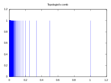
load(draw); /* by Mario Rodríguez Riotorto  http://riotorto.users.sourceforge.net/gnuplot/index.html  */

draw2d(
 title     = "Topologist\\47s comb", /* Syntax for postscript enhanced option; character 47 = '  */
 xrange        = [0.0,1.2],
 yrange        = [0,1.2],
 file_name = "comb2",
 terminal      = svg,
 points_joined = impulses, /* vertical segments are drawn from points to the x-axis  */
 color         = "blue",
 points(makelist(1/x,x,1,1000),makelist(1,y,1,1000)) )$
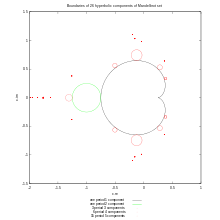
Example programs
- Iteration of complex numbers, stack and drawing a list of points
- Iteration of complex numbers, comparing complex numbers, finding period of cycle
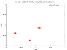
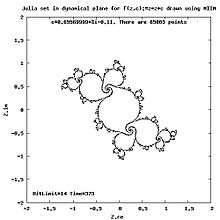
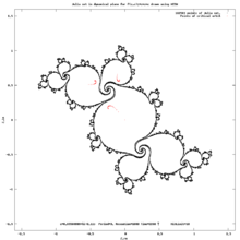
- Drawing Julia set and critical orbit. Computing period
- drawing curves in 2D plane
- drawing points
See also
- Images with Maxima CAS source code
- syntax highlight for Gedit
- questions tagged Maxima on stackoverflow
References
- ↑ Stackexchange : What are well-known weaknesses of CAS/math software?
- ↑ R Fateman : Branch Cuts in Computer Algebra,
- ↑ compiled deb packages for Maxima 5.20.1-1 by Istvan Blahota
- ↑ help from ubuntu community about Maxima
- ↑ How to build your own Maxima package by Andras Somogyi
- ↑ Install from Ubuntu repositories by Mario Rodriguez Riotorto
- ↑ launchpad : blahota wxmaxima
- ↑ How to build Maxima by Rupert Swarbrick
- ↑ [Maxima] Phantastic Program! One bug - discussion
- ↑ Discussion at Maxima interest list
- ↑ Maxima: Syntax improvements by Stavros Macrakis
- ↑ Maxima: what does Maxima call an “array”? - answer by Robert Dodier
- ↑ the Maxima mailing list : [Maxima] array and matrix? - answer by Robert Dodier
- ↑ Maxima Overview by Burkhard Bunk
- ↑ the Maxima mailing list : [Maxima] array and matrix? - answer by Robert Dodier
- ↑ Maxima Overview by Burkhard Bunk
- ↑ maxima manual : Category Matrices
- ↑ maxima manual : Package vect