Haskell/Understanding arrows

< Haskell

Arrows, like monads, express computations that happen within a context. However, they are a more general abstraction than monads, and thus allow for contexts beyond what the Monad class makes possible. The essential difference between the abstractions can be summed up thus:

Just as we think of a monadic type m a as representing a 'computation delivering an a '; so we think of an arrow type a b c, (that is, the application of the parameterised type a to the two parameters b and c) as representing 'a computation with input of type b delivering a c'; arrows make the dependence on input explicit.
—John Hughes, Generalising Monads to Arrows ^[1]

This chapter has two main parts. Firstly, we will consider the main ways in which arrow computations differ from those expressed by the functor classes we are used to, and also briefly present some of the core arrow-related type classes. Secondly, we will study the parser example used by John Hughes in the original presentation of arrows.

Pocket guide to `Arrow`

Arrows look a lot like functions

The first step towards understanding arrows is realising how similar they are to functions. Like (->), the type constructor of an Arrow instance has kind * -> * -> *, that is, it takes two type arguments − unlike, say, a Monad, which takes only one. Crucially, Arrow has Category as a superclass. Category is, to put it very roughly, the class for things that can be composed like functions:

class Category y where
    id  :: y a a -- identity for composition.
    (.) :: y b c -> y a b -> y a c -- associative composition.

(It goes without saying that functions have an instance of Category − in fact, they are Arrows as well.)

A practical consequence of this similarity is that you have to think in point-free terms when looking at expressions full of Arrow operators, such as this example from the tutorial:

(total &&& (const 1 ^>> total)) >>> arr (uncurry (/))

Otherwise you will quickly get lost looking for the values to apply things on. In any case, it is easy to get lost even if you look at such expressions in the right way. That's what proc notation is all about: adding extra variable names and whitespace while making some operators implicit, so that Arrow code gets easier to follow.

Before continuing, we should mention that Control.Category also defines (<<<) = (.) and (>>>) = flip (.), which is very commonly used to compose arrows from left to right.

`Arrow` glides between `Applicative` and `Monad`

In spite of the warning we gave just above, arrows can be compared to applicative functors and monads. The trick is making the functors look more like arrows, and not the opposite. That is, you should not compare Arrow y => y a b with Applicative f => f a or Monad m => m a, but rather with:

Applicative f => f (a -> b), the type of static morphisms i.e. the values to the left of (<*>); and
Monad m => a -> m b, the type of Kleisli morphisms i.e. the functions to the right of (>>=) ^[2].

Morphisms are the sort of things that can have Category instances, and indeed we could write instances of Category for both static and Kleisli morphisms. This modest twisting is enough for a sensible comparison.

If this argument reminds you of the sliding scale of power discussion, in which we compared Functor, Applicative and Monad, that is a sign you are paying attention, as we are following exactly the same route. Back then, we remarked how the types of the morphisms limit how they can, or cannot, create effects. Monadic binds can induce near-arbitrary changes to the effects of a computation depending on the a values given to the Kleisli morphism, while the isolation between the functorial wrapper and the function arrow in static morphisms mean the effects in an applicative computation do not depend at all on the values within the functor ^[3].

What sets arrows apart from this point of view is that in Arrow y => y a b there is no such connection between the context y and a function arrow to determine so rigidly the range of possibilities. Both static and Kleisli morphisms can be made into Arrows, and conversely an instance of Arrow can be made as limited as an Applicative one or as powerful as a Monad one ^[4]. More interestingly, we can use Arrow to take a third option and have both applicative-like static effects and monad-like dynamic effects in a single context, but kept separate from each other. Arrows make it possible to fine tune how effects are to be combined. That is the main thrust of the classic example of the arrow-based parser, which we will have a look at near the end of this chapter.

An `Arrow` can multitask

These are the Arrow methods:

class Category y => Arrow y where
    -- Minimal implementation: arr and first
    arr    :: (a -> b) -> y a b                 -- converts function to arrow
    first  :: y a b -> y (a, c) (b, c)          -- maps over first component

    second :: y a b -> y (c, a) (c, b)          -- maps over second component
    (***)  :: y a c -> y b d -> y (a, b) (c, d) -- first and second combined
    (&&&)  :: y a b -> y a c -> y a (b, c)      -- (***) on a duplicated value

With these methods, we can carry out multiple computations at each step of what seems to be a linear chain of composed arrows. That is done by keeping values used in separate computations as elements of pairs in a (possibly nested) pair, and then using the using pair-handling functions to reach each value when desired. That allows, for instance, saving intermediate values for later or using functions with multiple arguments conveniently ^[5].

Visualising may help understanding the data flow in an arrow computation. Here are illustrations of (>>>) and the five Arrow methods:

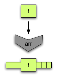
arr turns a function into an arrow, composable with other arrows. Naturally, not all arrows are created in this way.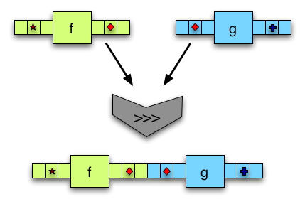
(>>>) composes two arrows. The output of the first one is fed to the second.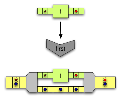
first takes two inputs side by side. The first one is modified using an arrow, while the second is left unchanged.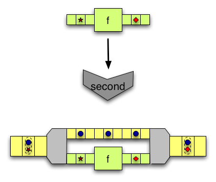
second, conversely, takes two inputs but only modifies the second.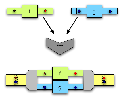
(***) takes two inputs and modifies them with two arrows, one for each input.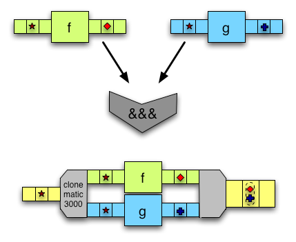
(&&&) takes one input, duplicates it and modifies each copy with a different arrow.

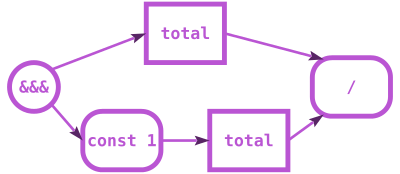
Data flow for the mean1 arrow from the tutorial. Rectangles are arrows, rounded rectangles are arrows made with arr, circles are other data flow split/merge points. Other combinators are left implicit. Corresponding code:

(total &&& (const 1 ^>> total))
    >>> arr (uncurry (/))

It is worth mentioning that Control.Arrow defines returnA = arr id as a do-nothing arrow. One of the arrow laws says returnA must be equivalent to the id from the Category instance ^[6].

An `ArrowChoice` can be resolute

If Arrow makes multitasking possible, ArrowChoice forces a decision on what task to do.

class Arrow y => ArrowChoice y where
    -- Minimal implementation: left
    left  :: y a b -> y (Either a c) (Either b c)          -- maps over left choice

    right :: y a b -> y (Either c a) (Either c b)          -- maps over right choice
    (+++) :: y a c -> y b d -> y (Either a b) (Either c d) -- left and right combined
    (|||) :: y a c -> y b c -> y (Either a b) c            -- (+++), then merge results

Either provides a way to tag the values, so that different arrows can handle them depending on whether they are tagged with Left or Right. Note that these methods involving Either are entirely analogous to those involving pairs offered by Arrow.

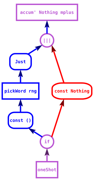
Data flow in a fragment of the getWord example of the tutorial. Blue indicates a Left tag and red indicates Right. Note that the if construct of proc notation sends True to Left and False to Right. Corresponding code:

proc () -> do
  firstTime <- oneShot -< ()
  mPicked <- if firstTime
    then do
      picked <- pickWord rng -< ()
      returnA -< Just picked
    else returnA -< Nothing
  accum' Nothing mplus -< mPicked

An `ArrowApply` is just boring

As the name suggests, ArrowApply makes it possible to apply arrows to values directly midway through an arrow computation. Ordinary Arrows do not allow that − we can just compose them on and on and on. Application only happens right at the end, once a run-arrow function of some sort is used to get a plain function from the arrow.

class Arrow y => ArrowApply y where
    app :: y (y a b, a) b -- applies first component to second

(For instance, app for functions is uncurry ($) = \(f, x) -> f x .)

app, however, comes at a steep price. Building an arrow as a value within an arrow computation and then eliminating it through application implies allowing the values within the computation to affect the context. That sounds a lot like what monadic binds do. It turns out that an ArrowApply is exactly equivalent to some Monad as long as the ArrowApply laws are followed. The ultimate consequence is that ArrowApply arrows cannot realise any of the interesting possibilities Arrow allows but Monad doesn't, such as having a partly static context.

The real flexibility with arrows comes with the ones that aren't monads, otherwise it's just a clunkier syntax.
—Philippa Cowderoy

Arrow combinators crop up in unexpected places

Functions are the trivial example of arrows, and so all of the Control.Arrow functions shown above can be used with them. For that reason, it is quite common to see arrow combinators being used in code that otherwise has nothing to do with arrows. Here is a summary of what they do with plain functions, alongside with combinators in other modules that can be used in the same way (in case you prefer the alternative names, or just prefer using simple modules for simple tasks).





Combinator
What it does
(specialised to (->))
Alternatives

(>>>) flip (.) 

first \f (x, y) -> (f x, y) first (Data.Bifunctor)

second \f (x, y) -> (x, f y) fmap; second (Data.Bifunctor)

(***) \f g (x, y) -> (f x, g y) bimap (Data.Bifunctor)

(&&&) \f g x -> (f x, g x) liftA2 (,) (Control.Applicative)

left Maps over Left case. first (Data.Bifunctor)

right Maps over Right case. fmap; second (Data.Bifunctor)

(+++) Maps over both cases. bimap (Data.Bifunctor)

(|||) Eliminates Either. either (Data.Either)

app \(f, x) -> f x uncurry ($)



The Data.Bifunctor module provides the Bifunctor class, of which pairs and Either are instances of. A Bifunctor is very much like a Functor, except that there are two independent ways of mapping functions over it, corresponding to the first and second methods ^[7].


Exercises

 Write implementations for second, (***) and (&&&). Use just (>>>), arr, and first (plus any plain functions) to implement second; after that, you can use the other combinators once you have implemented them.
 Write an implementation for right in terms of left.
 Implement liftY2 :: Arrow y =>
‌(a -> b -> c) -> y r a -> y r b -> y r c


 Using arrows 




 Avoiding leaks 

Arrows were originally motivated by an efficient parser design found by Swierstra & Duponcheel^[8].

To describe the benefits of their design, let's examine exactly how monadic parsers work.

If you want to parse a single word, you end up with several monadic parsers stacked end to end. Taking Parsec as an example ^[9], a parser for the string "word" can be thought of as ^[10]:


word = do char 'w' >> char 'o' >> char 'r' >> char 'd'
          return "word"


Each character is tried in order, if "worg" is the input, then the first three parsers will succeed, and the last one will fail, making the entire string "word" parser fail.

If you want to parse one of two options, you create a new parser for each and they are tried in order. The first one must fail in order for the next to be tried with the same input.


ab = char 'a' <|> char 'b' <|> char 'c' -- (<|>) is a combinator for alternatives.


To parse "c" successfully, both 'a' and 'b' must have been tried.


one = do char 'o' >> char 'n' >> char 'e'
      return "one"

two = do char 't' >> char 'w' >> char 'o'
      return "two"

three = do char 't' >> char 'h' >> char 'r' >> char 'e' >> char 'e'
        return "three"

nums = one <|> two <|> three


With these three parsers, you can't detect that the string "four" will fail the parser nums until the last parser has failed.

If one of the options can consume much of the input but will fail, you still must descend down the chain of parsers until the final parser fails. All of the input that can possibly be consumed by later parsers must be retained in memory in case one of them does consume it. That can lead to much more space usage than you would naively expect − a situation often called a space leak.

The general pattern with monadic parsers, then, is that each option must fail or one option must succeed.

 Can it be done better? 

Swierstra & Duponcheel (1996) noticed that a smarter parser could immediately fail upon seeing the very first character. For example, in the nums parser above, the choice of first letter parsers was limited to either the letter 'o' for "one" or the letter 't' for both "two" and "three". This smarter parser would also be able to garbage collect input sooner because it could look ahead to see if any other parsers might be able to consume the input, and drop input that could not be consumed. This new parser is a lot like the monadic parsers with the major difference that it exports static information. It's like a monad, but it also tells you what it can parse.

There's one major problem. This doesn't fit into the Monad interface. Monadic composition works with (a -> m b) functions, and functions alone. There's no way to attach static information. You have only one choice, throw in some input, and see if it passes or fails.

Back when this issue first arose, the monadic interface was being touted as a completely general purpose tool in the functional programming community, so finding that there was some particularly useful code that just couldn't fit into that interface was something of a setback.  This is where arrows come in.  John Hughes's Generalising monads to arrows proposed the arrows abstraction as new, more flexible tool.  

 Static and dynamic parsers 

Let us examine Swierstra and Duponcheel's parser in greater detail, from the perspective of arrows a presented by Hughes. The parser has two components: a fast, static parser which tells us if the input is worth trying to parse; and a slow, dynamic parser which does the actual parsing work.


import Control.Arrow
import qualified Control.Category as Cat
import Data.List (union)

data Parser s a b = P (StaticParser s) (DynamicParser s a b)
data StaticParser s = SP Bool [s]
newtype DynamicParser s a b = DP ((a, [s]) -> (b, [s]))


The static parser consists of a flag, which tells us if the parser can accept the empty input, and a list of possible starting characters.  For example, the static parser for a single character would be as follows:


spCharA :: Char -> StaticParser Char
spCharA c = SP False [c]


It does not accept the empty string (False) and the list of possible starting characters consists only of c.

The dynamic parser needs a little more dissecting. What we see is a function that goes from (a, [s]) to (b, [s]).  It is useful to think in terms of sequencing two parsers: each parser consumes the result of the previous parser (a), along with the remaining bits of input stream ([s]), it does something with a to produce its own result b, consumes a bit of string and returns that.  So, as an example of this in action, consider a dynamic parser (Int, String) -> (Int, String), where the Int represents a count of the characters parsed so far.  The table below shows what would happen if we sequence a few of them together and set them loose on the string "cake" :



result remaining

before 0 cake

after first parser 1 ake

after second parser 2 ke

after third parser 3 e



So the point here is that a dynamic parser has two jobs : it does something to the output of the previous parser (informally, a -> b), and it consumes a bit of the input string, (informally, [s] -> [s]), hence the type DP ((a,[s]) -> (b,[s])).  Now, in the case of a dynamic parser for a single character (type (Char, String) -> (Char, String)), the first job is trivial.  We ignore the output of the previous parser, return the character we have parsed and consume one character off the stream:


dpCharA :: Char -> DynamicParser Char Char Char
dpCharA c = DP (\(_,x:xs) -> (x,xs))


This might lead you to ask a few questions.  For instance, what's the point of accepting the output of the previous parser if we're just going to ignore it? And shouldn't the dynamic parser be making sure that the current character off the stream matches the character to be parsed by testing x == c?  The answer to the second question is no − and in fact, this is part of the point: the work is not necessary because the check would already have been performed by the static parser. Naturally, things are only so simple because we are testing just one character. If we were writing a parser for several characters in sequence we would need dynamic parsers that actually tested the second and further characters; and if we wanted to build an output string by chaining several parsers of characters then we would need the output of previous parsers.

Time to put both parsers together.  Here is our S+D style parser for a single character:


charA :: Char -> Parser Char Char Char
charA c = P (SP False [c]) (DP (\(_,x:xs) -> (x,xs)))


 Bringing the arrow combinators in 

With the preliminary bit of exposition done, we are now going to implement the Arrow class for Parser s, and by doing so, give you a glimpse of what makes arrows useful.  So let's get started:


-- We explain the Eq s constraint below.
instance Eq s => Arrow (Parser s) where


arr should convert an arbitrary function into a parsing arrow.  In this case, we have to use "parse" in a very loose sense: the resulting arrow accepts the empty string, and only the empty string (its set of first characters is []).  Its sole job is to take the output of the previous parsing arrow and do something with it.  That being so, it does not consume any input.


    arr f = P (SP True []) (DP (\(b,s) -> (f b,s)))


Likewise, the first combinator is relatively straightforward.  Given a parser, we want to produce a new parser that accepts a pair of inputs (b,d).  The first component of the input b, is what we actually want to parse.  The second part passes through untouched:


    first (P sp (DP p)) = P sp (DP (\((b,d),s) ->
        let (c, s') = p (b,s)
        in  ((c,d),s')))


We also have to supply the Category instance. id is entirely obvious, as id = arr id must hold:


instance Eq s => Cat.Category (Parser s) where
    id = P (SP True []) (DP (\(b,s) -> (b,s)))
    -- Or simply: id = P (SP True []) (DP id)


On the other hand, the implementation of (.) requires a little more thought.  We want to take two parsers, and return a combined parser incorporating the static and dynamic parsers of both arguments:


    -- The Eq s constraint is needed for using union here.
    (P (SP empty1 start1) (DP p2)) .
      (P (SP empty2 start2) (DP p1)) =
        P (SP (empty1 && empty2)
              (if not empty1 then start1 else start1 `union` start2))
          (DP (p2.p1))


Combining the dynamic parsers is easy enough; we just do function composition.  Putting the static parsers together requires a little bit of thought.  First of all, the combined parser can only accept the empty string if both parsers do.  Fair enough, now how about the starting symbols?  Well, the parsers are supposed to be in a sequence, so the starting symbols of the second parser shouldn't really matter.  If life were simple, the starting symbols of the combined parser would only be start1.  Alas, life is not simple, because parsers could very well accept the empty input.  If the first parser accepts the empty input, then we have to account for this possibility by accepting the starting symbols from both the first and the second parsers ^[11].




 So what do arrows buy us? 

If you look back at our Parser type and blank out the static parser section, you might notice that this looks a lot like the arrow instances for functions.


arr f = \(b, s) -> (f b, s)
first p = \((b, d), s) ->
            let (c, s') = p (b, s)
            in  ((c, d), s'))

id = id
p2 . p1 = p2 . p1


There's the odd s variable out for the ride, which makes the definitions look a little strange, but the outline of e.g. the simple first functions is there. Actually, what you see here is roughly the arrow instance for the State monad/Kleisli morphism (let f :: b -> c, p :: b -> State s c and (.) actually be (<=<) = flip (>=>)).

That's fine, but we could have easily done that with bind in classic monadic style, with first becoming just an odd helper function that could be easily written with a bit of pattern matching. But remember, our Parser type is not just the dynamic parser − it also contains the static parser.


arr f = SP True []
first sp = sp
(SP empty1 start1) >>> (SP empty2 start2) = (SP (empty1 && empty2)
        (if not empty1 then start1 else start1 `union` start2))


This is not at all a function, it's just pushing around some data types, and it cannot be expressed in a monadic way. But the Arrow interface can deal with just as well. And when we combine the two types, we get a two-for-one deal: the static parser data structure goes along for the ride along with the dynamic parser. The Arrow interface lets us transparently compose and manipulate the two parsers, static and dynamic, as a unit, which we can then run as a traditional, unified function.

 Arrows in practice  

Some examples of libraries using arrows:

 The Haskell XML Toolbox (project page and library documentation) uses arrows for processing XML. There is a Wiki page in the Haskell Wiki with a somewhat Gentle Introduction to HXT.
 Netwire (page library documentation) is a library for functional reactive programming (FRP). FRP is a functional paradigm for handling events and time-varying values, with use cases including user interfaces, simulations and games. Netwire has an arrow interface as well as an applicative one.
 Yampa (Haskell Wiki page library documentation) is another arrow-based FRP library, and a predecessor to Netwire.
 Hughes' arrow-style parsers were first described in his 2000 paper, but a usable implementation wasn't available until May 2005, when Einar Karttunen released PArrows.


 See also 

 Bibliography on arrows (haskell.org)

 Notes 

↑  The paper that introduced arrows. It is freely accessible through its publisher.
↑  Those two concepts are usually known as static arrows and Kleisli arrows respectively. Since using the word "arrow" with two subtly different meanings would make this text horribly confusing, we opted for "morphism", which is a synonym for this alternative meaning.
↑  Incidentally, that is why they are called static: the effects are set in stone by the sequencing of computations; the generated values cannot affect them.
↑  For details, see Idioms are oblivious, arrows are meticulous, monads are promiscuous, by Sam Lindley, Philip Wadler and Jeremy Yallop.
↑  "Conveniently" is arguably too strong a word, though, given how confusing handling nested tuples can get. Ergo, proc notation.
↑  Arrow has laws, and so do the other arrow classes we are discussing in these two chapters. We won't pause to pore over the laws here, but you can check them in the Control.Arrow documentation.
↑  Data.Bifunctor was only added to the core GHC libraries in version 7.10, so it might not be installed if you are using an older version. In that case, you can install the bifunctors package, which also includes several other bifunctor-related modules
↑  Swierstra, Duponcheel. Deterministic, error correcting parser combinators. 
↑  Parsec is a popular and powerful parsing library. See the parsec documentation on Hackage for more information.
↑  "Thought of as" because in actual code we evidently wouldn't return the string explicitly in such a crude way. Parsec offers a combinator string which would allow writing word = string "word". In any case, right now we are only concerned with how characters are tested, and so the crude parser is good enough for a mental model.
↑  A reasonable question at this point would be "Okay, we can compose the static parsers by uniting their lists, but when we are actually gone to test things with them?". The answer is that the static tests would be performed by the alternatives combinator, which unites two parsers to produce a parser that accepts input from either.

 Acknowledgements 

This module uses text from An Introduction to Arrows by Shae Erisson, originally written for The Monad.Reader 4

Combinator	What it does (specialised to `(->)`)	Alternatives
`(>>>)`	flip `(.)`
`first`	`\f (x, y) -> (f x, y)`	`first` (Data.Bifunctor)
`second`	`\f (x, y) -> (x, f y)`	`fmap`; `second` (Data.Bifunctor)
`(***)`	`\f g (x, y) -> (f x, g y)`	`bimap` (Data.Bifunctor)
`(&&&)`	`\f g x -> (f x, g x)`	`liftA2 (,)` (Control.Applicative)
`left`	Maps over `Left` case.	`first` (Data.Bifunctor)
`right`	Maps over `Right` case.	`fmap`; `second` (Data.Bifunctor)
`(+++)`	Maps over both cases.	`bimap` (Data.Bifunctor)
`(\|\|\|)`	Eliminates `Either`.	`either` (Data.Either)
`app`	`\(f, x) -> f x`	`uncurry ($)`

Exercises
Write implementations for `second`, `(***)` and `(&&&)`. Use just `(>>>)`, `arr`, and `first` (plus any plain functions) to implement `second`; after that, you can use the other combinators once you have implemented them. Write an implementation for `right` in terms of `left`. Implement `liftY2 :: Arrow y => ‌(a -> b -> c) -> y r a -> y r b -> y r c`

	result	remaining
before	0	cake
after first parser	1	ake
after second parser	2	ke
after third parser	3	e

This article is issued from Wikibooks. The text is licensed under Creative Commons - Attribution - Sharealike. Additional terms may apply for the media files.

Haskell/Understanding arrows

Pocket guide to Arrow

Arrows look a lot like functions

Arrow glides between Applicative and Monad

An Arrow can multitask

An ArrowChoice can be resolute

An ArrowApply is just boring

Arrow combinators crop up in unexpected places

Using arrows

Avoiding leaks

Can it be done better?

Static and dynamic parsers

Bringing the arrow combinators in

So what do arrows buy us?

Arrows in practice

See also

Notes

Acknowledgements

Pocket guide to `Arrow`

`Arrow` glides between `Applicative` and `Monad`

An `Arrow` can multitask

An `ArrowChoice` can be resolute

An `ArrowApply` is just boring