Fractals/Iterations in the complex plane/boettcher
< Fractals < Iterations in the complex planeIntro
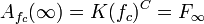
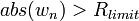
Exterior or complement of filled-in Julia set is :
- a basin of attraction of infinity ( superattracting fixed point) so dynamics in ttah basin is the same for all polynomials !!!
- one of components of the Fatou set
It can be analysed using
- escape time (simple but gives only radial values = escape time ) LSM/J,
- distance estimation ( more advanced, continuus, but gives only radial values = distance ) DEM/J
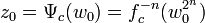
- Boettcher coordinate or complex potential ( the best )
" The dynamics of polynomials is much better understood than the dynamics of general rational maps" due to the Bottcher’s theorem[1]
Superattracting fixed points
For complex quadratic polynomial there are many superattracting fixed point ( with multiplier = 0 ):
- infinity ( It is always is superattracting fixed point for polynomials )
-
 is finite superattracting fixed point for map
- and
 are two finite superattracting fixed points for map
Description
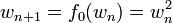
Near[2] super attracting fixed point (for example infinity) the behaviour of discrete dynamical system :
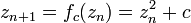
based on complex quadratic polynomial 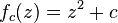 is similar to
based on 
It can be treated as one dynamical system viewed in two coordinate systems :
- easy ( w )
- hard to analyse( z )
In other words map  is conjugate [4] to map near infinity. [5]
History
In 1904 LE Boettcher :
- solved Schröder functional equation[6][7] in case of supperattracting fixed point[8]
- "proved the existence of an analytic function
 near
near  which conjugates the polynomial with
  , that is
  " ( Alexandre Eremenko ) [9]
Names
 is Boettcher function
where :

Complex potential on the parameter plane
Complex potential on dynamical plane
Complex potential or Boettcher coordinate has :
- radial values ( real potential ) LogPhi = CPM/J
- angular values ( external angle ) ArgPhi
Both values can be used to color with 2D gradient.
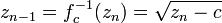
To compute Boettcher coordinate  use this formula [12]
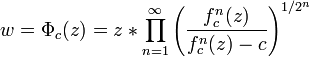
It looks "simple", but :
- square root of complex number gives two values so one have to choose one value
- more precision is needed near Julia set
LogPhi - Douady-Hubbard potential - real potential - radial component of complex potential
CPM/J

Note that potential inside Kc is zero so :
Pseudocode version :
if (LastIteration==IterationMax)
 then potential=0    /* inside  Filled-in Julia set */
 else potential= GiveLogPhi(z0,c,ER,nMax); /* outside */
It also removes potential error for log(0).
Full version
Math (full) notation : [13]
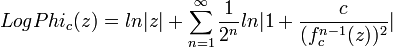
Maxima (full) function :
GiveLogPhi(z0,c,ER,nMax):=
block(
 [z:z0,
 logphi:log(cabs(z)),
 fac:1/2,
 n:0],
 while n<nMax and abs(z)<ER do
 (z:z*z+c,
 logphi:logphi+fac*log(cabs(1+c/(z*z))),
 n:n+1
 ),
 return(float(logphi))
)$
Simplified version
The escape rate function of a polynomial f is defined by :
where :

"The function Gp is continous on C and harmonic on the complement of the Julia set. It vanishes identically on K(f) and as it has a logarithmic pole at infinity, it is a it is the Green's function for C/ K(f)." ( Laura G. DeMarco) [14]
Math simplified formula :
Maxima function :
GiveSLogPhi(z0,c,e_r,i_max):=
 block(
  [z:z0,
   logphi,
   fac:1/2,
   i:0
  ],
  while i<i_max and cabs(z)<e_r do
  (z:z*z+c,
    fac:fac/2,
    i:i+1
  ),
 logphi:fac*log(cabs(z)),
 return(float(logphi))
)$
If you don't check if orbit is not bounded ( escapes, bailout test) then use this Maxima function :
GiveSLogPhi(z0,c,e_r,i_max):=
block(
 [z:z0, logphi, fac:1/2, i:0],
  while i<i_max and cabs(z)<e_r do
   (z:z*z+c,
    fac:fac/2,
    i:i+1 ),
   if i=i_max
    then logphi:0
    else logphi:fac*log(cabs(z)),
   float(logphi)
)$
C version :
double jlogphi(double zx0, double zy0, double cx, double cy)
/* this function is based on function by W Jung http://mndynamics.com */
{
 int j;
 double
 zx=zx0,
 zy=zy0,
 s = 0.5,
 zx2=zx*zx,
 zy2=zy*zy,
 t;
 for (j = 1; j < 400; j++)
 { s *= 0.5;
  zy = 2 * zx * zy + cy;
  zx = zx2 - zy2 + cx;
  zx2 = zx*zx;
  zy2 = zy*zy;
  t = fabs(zx2 + zy2); // abs(z)
  if ( t > 1e24) break;
 }
return s*log2(t);  // log(zn)* 2^(-n)
}//jlogphi
Euler version by R. Grothmann ( with small change : from z^2-c to z^2+c) :[15]
function iter (z,c,n=100) ...

h=z;
loop 1 to n;
h=h^2+c;
if totalmax(abs(h))>1e20; m=#; break; endif;
end;
return {h,m};
endfunction

x=-2:0.05:2; y=x'; z=x+I*y;
{w,n}=iter(z,c);
wr=max(0,log(abs(w)))/2^n;
Level Sets of potential = pLSM/J
Here is Delphi function which gives level of potential :
Function GiveLevelOfPotential(potential:extended):integer;
 var r:extended;
 begin
    r:= log2(abs(potential));
    result:=ceil(r);
 end;
ArgPhi - External angle - angular component of complex potential
One can start with binary decomposition of basin of attraction of infinity.
The second step can be using 
period detection
How to find period of external angle measured in turns under doubling map :
Here is Common Lisp code :
(defun give-period (ratio-angle)
  "gives period of angle in turns (ratio) under doubling map"
  (let* ((n (numerator ratio-angle))
	 (d (denominator ratio-angle))
	 (temp n)) ; temporary numerator

    (loop for p from 1 to 100 do
	  (setq temp  (mod (* temp 2) d)) ; (2 x n) modulo d = doubling)
	  when ( or (= temp n) (= temp 0)) return p )))
Maxima CAS code :
doubling_map(n,d):=mod(2*n,d);
/* catch-throw version by Stavros Macrakis, works */
GivePeriodOfAngle(n0,d):=
catch(
      block([ni:n0],
          for i thru 200 do if (ni:doubling_map(ni,d))=n0 then throw(i),
          0 ) )$


/* go-loop version, works */
GiveP(n0,d):=block(
[ni:n0,i:0],
block(
  loop,
  ni:doubling_map(ni,d),
  i:i+1,
  if i<100 and not (n0=ni) then go(loop)
),
if (n0=ni)
	then i
	else 0
);

/* Barton Willis while version without for loop , works */
GivePeriod(n0,d):=block([ni : n0,k : 1],
  while (ni : doubling_map(ni,d)) # n0 and k < 100 do (
    k : k + 1),
  if k = 100 then 0 else k)$
Computing external angle
External angle (argument) is argument of Boettcher coordinate

Because Boettcher coordinate is a product of complex numbers so argument of product is :
Constructing the spine of filled Julia set
Algorithm for constructiong the spine is described by A. Douady[16]
- join
 and
and  ,
, - (to do )
Drawing dynamic external ray
Field lines in in the Fatou domain
Explanation by Gert Buschmann
backwards iteration
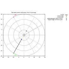
This method has been used by several people and proved by Thierry Bousch. [17]
Code in c++ by Wolf Jung can be found in procedure QmnPlane::backray() in file qmnplane.cpp ( see source code of the program Mandel ). [18]
- Ray for periodic angle ( simplest case )
It will be explained by an example :
First choose external angle  (in turns). External angle for periodic ray is a rational number.
Compute period of external angle under doubling map.
Because "1/3 doubled gives 2/3 and 2/3 doubled gives 4/3, which is congruent to 1/3" [19]
or
so external angle  has period 2 under doubling map.
Start with 2 points near infinity (in conjugate plane):
on ray 1/3 is a point 
on ray 2/3 is a point  .
.
Near infinity  so one can swith to dynamical plane ( Boettcher conjugation )
Backward iteration (with proper chose from two possibilities)[21] of point on ray 1/3 goes to ray 2/3, back to 1/3 and so on.
In C it is :
/* choose one of 2 roots: zNm1 or -zNm1  where zN = sqrt(zN - c )  */
if (creal(zNm1)*creal(zN) + cimag(zNm1)*cimag(zN) <= 0) zNm1=-zNm1;
or in Maxima CAS :
if (z1m1.z01>0) then z11:z1m1 else z11:-z1m1;
One has to divide set of points into 2 subsets ( 2 rays).
Draw one of these 2 sets and join the points. It will be an approximation of ray.
- Ray for preperiodic angle ( to do )
/*

compute last point ~ landing point
of the dynamic ray for periodic angles ( in turns )


 gcc r.c -lm -Wall -march=native


landing point of ray for angle = 1 / 15 = 0.0666666666666667 is = (0.0346251977103306 ;  0.4580500411138030 ) ; iDistnace = 18
landing point of ray for angle = 2 / 15 = 0.1333333333333333 is = (0.0413880816505388 ;  0.5317194187688231 ) ; iDistnace = 17
landing point of ray for angle = 4 / 15 = 0.2666666666666667 is = (-0.0310118081927549 ;  0.5440125864026020 ) ; iDistnace = 17
landing point of ray for angle = 8 / 15 = 0.5333333333333333 is = (-0.0449867688014234 ;  0.4662592852362425 ) ; iDistnace = 18


*/

// https://gitlab.com/adammajewski/ray-backward-iteration
#include <stdio.h>
#include <stdlib.h> // malloc
#include <math.h> // M_PI; needs -lm also
#include <complex.h>

/* --------------------------------- global variables and consts ------------------------------------------------------------ */
#define iPeriodChild 4 // iPeriodChild of secondary component joined by root point


// - --------------------- functions ------------------------


/*
   principal square  root of complex number
   wikipedia  Square_root

   z1= I;
   z2 = root(z1);
   printf("zx  = %f \n", creal(z2));
   printf("zy  = %f \n", cimag(z2));
*/
double complex root(double x, double y)
{

  double u;
  double v;
  double r = sqrt(x*x + y*y);

  v = sqrt(0.5*(r - x));
  if (y < 0) v = -v;
  u = sqrt(0.5*(r + x));
  return u + v*I;
}


// This function only works for periodic  angles.
// You must know the iPeriodChild n before calling this function.
// draws all "iPeriodChild" external rays
// commons  File:Backward_Iteration.svg
// based on the code by Wolf Jung from program Mandel
// http://www.mndynamics.com/

int ComputeRays( //unsigned char A[],
			    int n, //iPeriodChild of ray's angle under doubling map
			    int iterMax,
                            double Cx,
                            double Cy,
                            double dAlfaX,
                            double dAlfaY,
                            double PixelWidth,
                            complex double zz[iPeriodChild] // output array

			    )
{
  double xNew; // new point of the ray
  double yNew;

  const double R = 10000; // very big radius = near infinity
  int j; // number of ray
  int iter; // index of backward iteration

  double t,t0; // external angle in turns
  double num, den; // t = num / den

  double complex zPrev;
  double u,v; // zPrev = u+v*I

  int iDistance ; // dDistance/PixelWidth = distance to fixed in pixels


  /* dynamic 1D arrays for coordinates ( x, y) of points with the same R on preperiodic and periodic rays  */
  double *RayXs, *RayYs;
  int iLength = n+2; // length of arrays ?? why +2


  //  creates arrays :  RayXs and RayYs  and checks if it was done
  RayXs = malloc( iLength * sizeof(double) );
  RayYs = malloc( iLength * sizeof(double) );
  if (RayXs == NULL || RayYs==NULL)
    {
      fprintf(stderr,"Could not allocate memory");
      getchar();
      return 1; // error
    }


   // external angle of the first ray
   num = 1.0;
   den = pow(2.0,n) -1.0;
   t0 = num/den; // http://fraktal.republika.pl/mset_external_ray_m.html
   t=t0;
   // printf(" angle t = %.0f / %.0f = %f in turns \n", num, den, t0);


  //  starting points on preperiodic and periodic rays
  //  with angles t, 2t, 4t...  and the same radius R
  for (j = 0; j < n; j++)
    { // z= R*exp(2*Pi*t)
      RayXs[j] = R*cos((2*M_PI)*t);
      RayYs[j] = R*sin((2*M_PI)*t);
      //
      // printf(" %d angle t = = %.0f / %.0f =  %.16f in turns \n", j, num , den,  t);
      //
      num *= 2.0;
      t *= 2.0; // t = 2*t
      if (t > 1.0) t--; // t = t modulo 1

    }
  //zNext = RayXs[0] + RayYs[0] *I;

  // printf("RayXs[0]  = %f \n", RayXs[0]);
  // printf("RayYs[0]  = %f \n", RayYs[0]);

  // z[k] is n-periodic. So it can be defined here explicitly as well.
  RayXs[n] = RayXs[0];
  RayYs[n] = RayYs[0];


  //   backward iteration of each point z
  for (iter = -10; iter <= iterMax; iter++)
    {

      for (j = 0; j < n; j++) // n +preperiod
	{ // u+v*i = sqrt(z-c)   backward iteration in fc plane
	  zPrev = root(RayXs[j+1] - Cx , RayYs[j+1] - Cy ); // , u, v
	  u=creal(zPrev);
	  v=cimag(zPrev);

	  // choose one of 2 roots: u+v*i or -u-v*i
	  if (u*RayXs[j] + v*RayYs[j] > 0)
	    { xNew = u; yNew = v; } // u+v*i
	  else { xNew = -u; yNew = -v; } // -u-v*i


	  // draw part of the ray = line from zPrev to zNew
	 // dDrawLine(A, RayXs[j], RayYs[j], xNew, yNew, j, 255);


	  //
	  RayXs[j] = xNew; RayYs[j] = yNew;


	} // for j ...

          //RayYs[n+k] cannot be constructed as a preimage of RayYs[n+k+1]
      RayXs[n] = RayXs[0];
      RayYs[n] = RayYs[0];

      // convert to pixel coordinates
      //  if z  is in window then draw a line from (I,K) to (u,v) = part of ray

      // printf("for iter = %d cabs(z) = %f \n", iter, cabs(RayXs[0] + RayYs[0]*I));

    }

  // aproximate end of ray by straight line to it's landing point here = alfa fixed point
 // for (j = 0; j < n + 1; j++)
  //  dDrawLine(A, RayXs[j],RayYs[j], dAlfaX, dAlfaY,j, 255 );


  // this check can be done only from inside this function
  t=t0;
  num = 1.0;
  for (j = 0; j < n ; j++)
    {

      zz[j] = RayXs[j] +  RayYs[j] * I; // save to the output array
      // aproximate end of ray by straight line to it's landing point here = alfa fixed point
      //dDrawLine(RayXs[j],RayYs[j], creal(alfa), cimag(alfa), 0, data);
      iDistance = (int) round(sqrt((RayXs[j]-dAlfaX)*(RayXs[j]-dAlfaX) +  (RayYs[j]-dAlfaY)*(RayYs[j]-dAlfaY))/PixelWidth);
      printf("last point of the ray for angle = %.0f / %.0f = %.16f is = (%.16f ;  %.16f ) ; Distance to fixed = %d  pixels \n",num, den, t, RayXs[j], RayYs[j],  iDistance);
      num *= 2.0;
      t *= 2.0; // t = 2*t
      if (t > 1) t--; // t = t modulo 1
    } // end of the check


  // free memmory
  free(RayXs);
  free(RayYs);


  return  0; //
}


int main()
{

  complex double l[iPeriodChild];
  int i;
  // external angle in turns = num/den;
  double num = 1.0;
  double den = pow(2.0, iPeriodChild) -1.0;

   ComputeRays( iPeriodChild,
                   10000,
                   0.25, 0.5,
                   0.00, 0.5,
                   0.003,
                   l ) ;


  printf("\n see what is in the output array : \n");

  for (i = 0; i < iPeriodChild ; i++) {
       printf("last point of the ray for angle = %.0f / %.0f = %.16f is = (%.16f ;  %.16f ) \n",num, den, num/den, creal(l[i]), cimag(l[i]));
       num *= 2.0;}


  return 0;
}
Run it :
./a.out
And output :
last point of the ray for angle = 1 / 15 = 0.0666666666666667 is = (0.0346251977103306 ;  0.4580500411138030 ) ; Distance to fixed = 18  pixels
last point of the ray for angle = 2 / 15 = 0.1333333333333333 is = (0.0413880816505388 ;  0.5317194187688231 ) ; Distance to fixed = 17  pixels
last point of the ray for angle = 4 / 15 = 0.2666666666666667 is = (-0.0310118081927549 ;  0.5440125864026020 ) ; Distance to fixed = 18  pixels
last point of the ray for angle = 8 / 15 = 0.5333333333333333 is = (-0.0449867688014234 ;  0.4662592852362425 ) ; Distance to fixed = 19  pixels

 see what is in the output array :
last point of the ray for angle = 1 / 15 = 0.0666666666666667 is = (0.0346251977103306 ;  0.4580500411138030 )
last point of the ray for angle = 2 / 15 = 0.1333333333333333 is = (0.0413880816505388 ;  0.5317194187688231 )
last point of the ray for angle = 4 / 15 = 0.2666666666666667 is = (-0.0310118081927549 ;  0.5440125864026020 )
last point of the ray for angle = 8 / 15 = 0.5333333333333333 is = (-0.0449867688014234 ;  0.4662592852362425 )
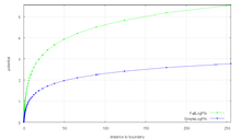
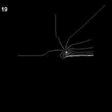
Point on the ray is moving backwards:
- very fast when it it far from Julia set
- very slow near Julia set ( after 50 iterations distance between points = 0 pixels )
See example computing ( here pixel size = 0.003 ) :
# iteration distance_between_points_in_pixels
0 	 3300001
1 	 30007
2 	 2296
3 	 487
4 	 179
5 	 92
6 	 54
7 	 34
8 	 23
9 	 18
10 	 14
11 	 11
12 	 9
13 	 7
14 	 6
15 	 5
16 	 5
17 	 4
18 	 4
19 	 3
20 	 3
21 	 3
22 	 3
23 	 2
24 	 2
25 	 2
26 	 2
27 	 2
28 	 2
29 	 2
30 	 1
31 	 1
32 	 1
33 	 1
34 	 1
35 	 1
36 	 1
37 	 1
38 	 1
39 	 1
40 	 1
41 	 1
42 	 1
43 	 1
44 	 1
45 	 1
46 	 1
47 	 1
48 	 1
49 	 1
50 	 1
51 	 1
52 	 1
53 	 1
54 	 1
55 	 1
56 	 0
57 	 0
58 	 0
59 	 0
60 	 0
One can choose points which differ by pixel size :
#iteration    distance(z1,z2)   distance (z,alfa)
       0 	 3300001 	 33368
       1 	   30007 	  3364
       2 	    2296 	  1074
       3 	     487 	   591
       4 	     179 	   413
       5 	      92 	   321
       6 	      54 	   267
       7 	      34 	   234
       8 	      23 	   211
       9 	      18 	   193
      10 	      14 	   179
      11 	      11 	   169
      12 	       9 	   160
      13 	       7 	   153
      14 	       6 	   146
      15 	       5 	   141
      16 	       5 	   136
      17 	       4 	   132
      18 	       4 	   128
      19 	       3 	   125
      20 	       3 	   122
      21 	       3 	   119
      22 	       3 	   117
      23 	       2 	   115
      24 	       2 	   112
      25 	       2 	   110
      26 	       2 	   109
      27 	       2 	   107
      28 	       2 	   105
      29 	       2 	   104
      30 	       1 	   102
      31 	       1 	   101
      32 	       1 	   100
      33 	       1 	    99
      34 	       1 	    97
      35 	       1 	    96
      36 	       1 	    95
      38 	       2 	    93
      40 	       2 	    92
      42 	       2 	    90
      44 	       2 	    88
      46 	       1 	    87
      48 	       1 	    86
      50 	       1 	    84
      52 	       1 	    83
      54 	       1 	    82
      56 	       1 	    81
      59 	       1 	    80
      62 	       1 	    78
      65 	       1 	    77
      68 	       1 	    76
      71 	       1 	    75
      74 	       1 	    74
      78 	       1 	    73
      82 	       1 	    71
      86 	       1 	    70
      90 	       1 	    69
      95 	       1 	    68
     100 	       1 	    67
     105 	       1 	    66
     111 	       1 	    65
     117 	       1 	    64
     124 	       1 	    63
     131 	       1 	    62
     139 	       1 	    60
     147 	       1 	    59
     156 	       1 	    58
     166 	       1 	    57
     177 	       1 	    56
     189 	       1 	    55
     202 	       1 	    54
     216 	       1 	    53
     231 	       1 	    52
     247 	       1 	    51
     265 	       1 	    50
     285 	       1 	    49
     307 	       1 	    48
     331 	       1 	    47
     358 	       1 	    46
     388 	       1 	    45
     421 	       1 	    44
     458 	       1 	    43
     499 	       1 	    42
     545 	       1 	    41
     597 	       1 	    40
     655 	       1 	    39
     721 	       1 	    38
     796 	       1 	    37
     881 	       1 	    36
     978 	       1 	    35
    1090 	       1 	    34
    1219 	       1 	    33
    1368 	       1 	    32
    1542 	       1 	    31
    1746 	       1 	    30
    1986 	       1 	    29
    2270 	       1 	    28
    2608 	       1 	    27
    3013 	       1 	    26
    3502 	       1 	    25
    4098 	       1 	    24
    4830 	       1 	    23
    5737 	       1 	    22
    6873 	       1 	    21
    8312 	       1 	    20
   10157 	       1 	    19
   12555 	       1 	    18
   15719 	       1 	    17
   19967 	       1 	    16
   25780 	       1 	    15
   33911 	       1 	    14
   45574 	       1 	    13
   62798 	       1 	    12
   89119 	       1 	    11
  131011 	       1 	    10
  201051 	       1 	     9
  325498 	       1 	     8
  564342 	       1 	     7
 1071481 	       1 	     6
 2308074 	       1 	     5
 5996970 	       1 	     4
21202243 	       1 	     3
136998728 	       1 	     2
One can see that moving from pixel 12 to 11 near alfa needs 27 000 iterations. Computing points up to 1 pixel near alfa needs : 2m1.236s
Drawing dynamic external ray using inverse Boettcher map by Curtis McMullen
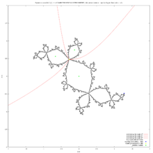
This method is based on C program by Curtis McMullen[22] and its Pascal version by Matjaz Erat[23]
There are 2 planes[24]here :
- w-plane ( or f0 plane )
- z-plane ( dynamic plane of fc plane )
Method consist of 3 big steps :
- compute some w-points of external ray of circle for angle
 and various radii (rasterisation)
 where
where 
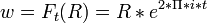
- map w-points to z-point using inverse Boettcher map

- draw z-points ( and connect them using segments ( line segment is a part of a line that is bounded by two distinct end points[25] )
First and last steps are easy, but second is not so needs more explanation.
Rasterisation
For given external ray in plane each point of ray has :
- constant value ( external angle in turns )
- variable radius

so points of ray are parametrised by radius
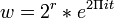
and can be computed using exponential form of complex numbers :
One can go along ray using linear scale :
t:1/3; /* example value */
R_Max:4;
R_Min:1.1;
for R:R_Max step -0.5 thru R_Min do w:R*exp(2*%pi*%i*t);
/* Maxima allows non-integer values in for statement */
It gives some w points with equal distance between them.
Another method is to use nonlinera scale.
To do it we introduce floating point exponent  such that :

and
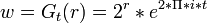
To compute some w points of external ray in plane for angle use
such Maxima code :
t:1/3; /* external angle in turns */
/* range for computing  R ; as r tends to 0 R tends to 1 */
rMax:2; /* so Rmax=2^2=4 /
rMin:0.1; /* rMin > 0   */
caution:0.93; /* positive number < 1 ; r:r*caution  gives smaller r */
r:rMax;
unless r<rMin do
(
 r:r*caution, /* new smaller r */
 R:2^r, /* new smaller R */
 w:R*exp(2*%pi*%i*t) /* new point w in f0 plane */
);
In this method distance between points is not equal but inversely proportional to distance to boundary of filled Julia set.
It is good because here ray has greater curvature so curve will be more smooth.
Mapping
Mapping points from to consist of 4 minor steps :
- forward iteration in plane
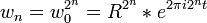
until  is near infinity
- switching plane ( from to )

( because here, near infinity :  )
)
- backward iteration in plane the same (
 ) number of iterations
 - last point
 is on our external ray
1,2 and 4 minor steps are easy. Third is not.
Backward iteration uses square root of complex number. It is 2-valued functions so backward iteration gives binary tree.
One can't choose good path in such tree without extre informations. To solve it we will use 2 things :
- equicontinuity of basin of attraction of infinity
- conjugacy between and planes
Equicontinuity of basin of attraction of infinity
Basin of attraction of infinity ( complement of filled-in Julia set) contains all points which tends to infinity under forward iteration.

Infinity is superattracting fixed point and orbits of all points have similar behaviour. In other words orbits of 2 points are assumed to stay close if they are close at the beginning.
It is equicontinuity ( compare with normality).
In plane one can use forward orbit of previous point of ray for computing backward orbit of next point.
Detailed version of algorithm
- compute first point of ray (start near infinity ang go toward Julia set )
 where
where 
here one can easily switch planes :
It is our first z-point of ray.
- compute next z-point of ray
- compute next w-point of ray for

- compute forward iteration of 2 points : previous z-point and actual w-point. Save z-orbit and last w-point
- switch planes and use last w-point as a starting point :

- backward iteration of new
 toward new using forward orbit of previous z point
 - is our next z point of our ray
- compute next w-point of ray for
- and so on ( next points ) until

Maxima CAS src code
/* gives a list of z-points of external ray for angle t in turns and coefficient c */
GiveRay(t,c):=
block(
 [r],
 /* range for drawing  R=2^r ; as r tends to 0 R tends to 1 */
 rMin:1E-20, /* 1E-4;  rMin > 0  ; if rMin=0 then program has infinity loop !!!!! */
 rMax:2,
 caution:0.9330329915368074, /* r:r*caution ; it gives smaller r */
 /* upper limit for iteration */
 R_max:300,
 /* */
 zz:[], /* array for z points of ray in fc plane */
 /*  some w-points of external ray in f0 plane  */
 r:rMax,
 while 2^r<R_max do r:2*r, /* find point w on ray near infinity (R>=R_max) in f0 plane */
 R:2^r,
 w:rectform(ev(R*exp(2*%pi*%i*t))),
 z:w, /* near infinity z=w */
 zz:cons(z,zz),
 unless r<rMin do
 ( /* new smaller R */
  r:r*caution,
  R:2^r,
  /* */
  w:rectform(ev(R*exp(2*%pi*%i*t))),
  /* */
  last_z:z,
  z:Psi_n(r,t,last_z,R_max), /* z=Psi_n(w) */
  zz:cons(z,zz)
 ),
 return(zz)
)$
Lamination of dynamical plane
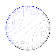
Here is long description
See also
References
- ↑ ON THE NOTIONS OF MATING by CARSTEN LUNDE PETERSEN AND DANIEL MEYER
- ↑ Neighbourhood in wikipedia
- ↑ The work of George Szekeres on functional equations by Keith Briggs
- ↑ Topological conjugacy in wikipedia
- ↑ How to draw external rays by Wolf Jung
- ↑ Schröder equation in wikipedia
- ↑ Lucjan Emil Böttcher and his mathematical legacy by Stanislaw Domoradzki, Malgorzata Stawiska
- ↑ L. E. Boettcher, The principal laws of convergence of iterates and their aplication to analysis (Russian), Izv. Kazan. fiz.-Mat. Obshch. 14) (1904), 155-234.
- ↑ Mathoverflow : Growth of the size of iterated polynomials
- ↑ Böttcher equation at Hyperoperations Wiki
- ↑ wikipedia : Böttcher's equation
- ↑ How to draw external rays by Wolf Jung
- ↑ The Beauty of Fractals, page 65
- ↑ Holomorphic families of rational maps: dynamics, geometry, and potential theory. A thesis presented by Laura G. DeMarco
- ↑ Euler examples by R. Grothmann
- ↑ A. Douady, “Algorithms for computing angles in the Mandelbrot set,” in Chaotic Dynamics and Fractals, M. Barnsley and S. G. Demko, Eds., vol. 2 of Notes and Reports in Mathematics in Science and Engineering, pp. 155–168, Academic Press, Atlanta, Ga, USA, 1986.
- ↑ Thierry Bousch : De combien tournent les rayons externes? Manuscrit non publié, 1995
- ↑ Program Mandel by Wolf Jung
- ↑ Explanation by Wolf Jung
- ↑ Modular arithmetic in wikipedia
- ↑ Square root of complex number gives 2 values so one has to choose only one. For details see Wolf Jung page
- ↑ c program by Curtis McMullen (quad.c in Julia.tar.gz)
- ↑ Quadratische Polynome by Matjaz Erat
- ↑ wikipedia : Complex_quadratic_polynomial / planes / Dynamical_plane
- ↑ wikipedia : Line segment