Fractals/Iterations in the complex plane/Mandelbrot set/boundary

< Fractals < Iterations in the complex plane < Mandelbrot set

Intro

Boundary of Mandelbrot set consist of :^[1]

boundaries of primitive and satellite hyperbolic components of Mandelbrot set including points :
- Parabolic (including 1/4 and primitive roots which are landing points for 2 parameter rays with rational external angles = biaccesible ).
- Siegel ( a unique parameter ray landing with irrational external angle)
- Cremer ( a unique parameter ray landing with irrational external angle)
Boundary of M without boundaries of hyperbolic components with points
- non-renormalizable (Misiurewicz with rational external angle and other).
- finitely renormalizable (Misiurewicz and other).
- infinitely renormalizble (Feigenbaum and other). Angle in turns of external rays landing on the Feigenbaum point are irrational numbers
boundaries of non hyperbolic components ( we believe they do not exist but we cannot prove it ) Boundaries of non-hyperbolic components would be infinitely renormalizable as well.

Boundary of Mandelbrot set as an image of unit circle under

\Psi _{M}\,

Mini Mandelbrot sets

midget = mini mandelbrot set = primitive component ( ?)

Parameter rays of mini Mandelbrot sets ^[2]

" a saddle-node (parabolic) periodic point in a complex dynamical system often admits homoclinic points, and in the case that these homoclinic points are nondegenerate, this is accompanied by the existence of infinitely many baby Mandelbrot sets converging to the saddle-node parameter value in the corresponding parameter plane." Devaney ^[3]

Drawing boundaries

Methods used to draw boundary of Mandelbrot set :^[4]

whole boundary
- Distance Estimation Method for Mandelbrots set = DEM/M ( exterior, interior or both)
- Boundary scanning method (BSM) : detecting the edges after Boolean escape time ^[5]
- boundary tracing method ^[6]^[7]
- contour integration by Robert Davies^[8]
- Jungreis function^[9] $\Psi _{M}\,$
drawing boundaries of components of Mandelbrot set
- Newton method

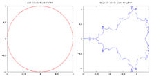
How to draw whole M set boundary

Jungreis function $\Psi _{M}\,$

Boundary of Mandelbrot set as an image of unit circle under Jungreis function

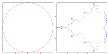
Description :

Drawing Mc by Jungreis Algorithm ^[10]
Maxima CAS src code ^[11]

Python code

#!/usr/bin/env python
"""
    Python code by Matthias Meschede 2014
    http://pythology.blogspot.fr/2014/08/parametrized-mandelbrot-set-boundary-in.html
"""
import numpy as np
import matplotlib.pyplot as plt

nstore = 3000  #cachesize should be more or less as high as the coefficients
betaF_cachedata = np.zeros( (nstore,nstore))
betaF_cachemask = np.zeros( (nstore,nstore),dtype=bool)
def betaF(n,m):
    """
    This function was translated to python from
    http://fraktal.republika.pl/mset_jungreis.html
    It computes the Laurent series coefficients of the jungreis function
    that can then be used to map the unit circle to the Mandelbrot
    set boundary. The mapping of the unit circle can also
    be seen as a Fourier transform. 
    I added a very simple global caching array to speed it up
    """
    global betaF_cachedata,betaF_cachemask

    nnn=2**(n+1)-1
    if betaF_cachemask[n,m]:
        return betaF_cachedata[n,m]
    elif m==0:
        return 1.0
    elif ((n>0) and (m < nnn)):
        return 0.0
    else: 
        value = 0.
        for k in range(nnn,m-nnn+1):
            value += betaF(n,k)*betaF(n,m-k)
        value = (betaF(n+1,m) - value - betaF(0,m-nnn))/2.0 
        betaF_cachedata[n,m] = value
        betaF_cachemask[n,m] = True
        return value

def main():
    #compute coefficients (reduce ncoeffs to make it faster)
    ncoeffs= 2400
    coeffs = np.zeros( (ncoeffs) )
    for m in range(ncoeffs):
        if m%100==0: print '%d/%d'%(m,ncoeffs)
        coeffs[m] = betaF(0,m+1)

    #map the unit circle  (cos(nt),sin(nt)) to the boundary
    npoints = 10000
    points = np.linspace(0,2*np.pi,npoints)
    xs     = np.zeros(npoints)
    ys     = np.zeros(npoints)
    xs = np.cos(points)
    ys = -np.sin(points)
    for ic,coeff in enumerate(coeffs):
        xs += coeff*np.cos(ic*points)
        ys += coeff*np.sin(ic*points)
    
    #plot the function
    plt.figure()
    plt.plot(xs,ys)
    plt.show()

if __name__ == "__main__":
    main()

How to draw boundaries of hyperbolic components

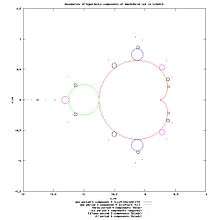
Boundaries of hyperbolic components for periods 1-6 as a solutions of boundary equations

Methods of drawing boundaries:

solving boundary equations :
- using method by Brown,Stephenson,Jung . It works only up to period 7-8 ^[12]
- using resultants ^[13]
parametrisation of boundary with Newton method near centers of components^[14] ^[15]. This methods needs centers, so it has some limitations,

Boundary scanning : detecting the edges after detecting period by checking every pixel. This method is slow but allows zooming. Draws "all" components
Boundary tracing for given c value. Draws single component.
Fake Mandelbrot set by Anne M. Burns : draws main cardioid and all its descendants. Do not draw mini Mandelbrot sets. ^[16]

"... to draw the boundaries of hyperbolic components using Newton's method. That is, take a point in the hyperbolic component that you are interested in (where there is an attracting cycle), and then find a curve along which the modulus of the multiplier tends to one. Then you will have found an indifferent parameter. Now you can similarly change the argument of the multiplier, again using Newton's method, and trace this curve. Some care is required near "cusps". " Lasse Rempe-Gillen^[17]

solving boundary equations

System of 2 equations defining boundaries of period $n\,$ hyperbolic components

first defines periodic point,
second defines indifferent orbit ( multiplier of periodic point is equal to one ).

${\begin{cases}F(n,z,c)=z\\abs(\lambda (z))=1\end{cases}}$

Because stability index $abs(\lambda )\,$ is equal to radius of point of unit circle $abs(w)\,$ :

$abs(\lambda )=abs(w)\,$

so one can change second equation to form ^[18] :

$\lambda =w\,$

It gives system of equations :

${\begin{cases}F(n,z,c)=z\\\lambda =w\end{cases}}$

It can be used for :

drawing components ( boundaries, internal rays )
finding indifferent parameters ( parabolic or for Siegel discs )

Above system of 2 equations has 3 variables : $z,c,w\,$ ( $n\,$ is constant and multiplier $\lambda \,$ is a function of $z,c\,$ ). One have to remove 1 variable to be able to solve it.

Boundaries are closed curves : cardioids or circles. One can parametrize points of boundaries with angle $t\,$ ( here measured in turns from 0 to 1 ).

After evaluation of $w=l(t)\,$ one can put it into above system, and get a system of 2 equations with 2 variables $z,c\,$ .

Now it can be solved

For periods:

1-3 it can be solved with symbolical methods and give implicit ( boundary equation) $b_{p}(w,c)=0\,$ and explicit function (inverse multiplier map) : $c=\gamma _{p}(w)\,$
- 1-2 it is easy to solve ^[19]
- 3 it can be solve using "elementary algebra" ( Stephenson )
>3 it can't be reduced to explicitly function but
- can be reduced to implicit solution ( boundary equation) $b_{p}(w,c)=0\,$ and solved numerically
- can be solved numerically using Newton method for solving system of nonlinear equations

Solving system of equation for period 1

Here is Maxima code :

(%i4) p:1;
(%o4) 1
(%i5) e1:F(p,z,c)=z;
(%o5) z^2+c=z
(%i6) e2:m(p)=w;
(%o6) 2*z=w
(%i8) s:eliminate ([e1,e2], [z]);
(%o8) [w^2-2*w+4*c]
(%i12) s:solve([s[1]], [c]);
(%o12) [c=-(w^2-2*w)/4]
(%i13) define (m1(w),rhs(s[1]));
(%o13) m1(w):=-(w^2-2*w)/4

Second equation contains only one variable, one can eliminate this variable. Because boundary equation is simple so it is easy to get explicit solution

m1(w):=-(w^2-2*w)/4

Solving system of equation for period 2

Here is Maxima code using to_poly_solve package by Barton Willis:

(%i4) p:2;
(%o4) 2
(%i5) e1:F(p,z,c)=z;
(%o5) (z^2+c)^2+c=z
(%i6) e2:m(p)=w;
(%o6) 4*z*(z^2+c)=w
(%i7) e1:F(p,z,c)=z;
(%o7) (z^2+c)^2+c=z
(%i10) load(topoly_solver);
to_poly_solve([e1, e2], [z, c]);
(%o10) C:/PROGRA~1/MAXIMA~1.1/share/maxima/5.16.1/share/contrib/topoly_solver.mac
(%o11) [[z=sqrt(w)/2,c=-(w-2*sqrt(w))/4],[z=-sqrt(w)/2,c=-(w+2*sqrt(w))/4],[z=(sqrt(1-w)-1)/2,c=(w-4)/4],[z=-(sqrt(1-w)+1)/2,c=(w-4)/4]]
(%i12) s:to_poly_solve([e1, e2], [z, c]);
(%o12) [[z=sqrt(w)/2,c=-(w-2*sqrt(w))/4],[z=-sqrt(w)/2,c=-(w+2*sqrt(w))/4],[z=(sqrt(1-w)-1)/2,c=(w-4)/4],[z=-(sqrt(1-w)+1)/2,c=(w-4)/4]]
(%i14) rhs(s[4][2]);
(%o14) (w-4)/4
(%i16) define (m2 (w),rhs(s[4][2]));
(%o16) m2(w):=(w-4)/4

explicit solution :

m2(w):=(w-4)/4

Solving system of equation for period 3

For period 3 ( and higher) previous method give no results (Maxima code) :

(%i14) p:3;
e1:z=F(p,z,c);
e2:m(p)=w;
load(topoly_solver);
to_poly_solve([e1, e2], [z, c]);
(%o14) 3
(%o15) z=((z^2+c)^2+c)^2+c
(%o16) 8*z*(z^2+c)*((z^2+c)^2+c)=w
(%i17) 
(%o17) C:/PROGRA~1/MAXIMA~1.1/share/maxima/5.16.1/share/contrib/topoly_solver.mac
`algsys' cannot solve - system too complicated.
#0: to_poly_solve(e=[z = ((z^2+c)^2+c)^2+c,8*z*(z^2+c)*((z^2+c)^2+c) = w],vars=[z,c])
-- an error.  To debug this try debugmode(true);

I use code by Robert P. Munafo^[20] which is based on paper of Wolf Jung.

One can approximate period 3 components with equations ^[21] :

(%i1) z:x+y*%i;
(%o1)                              %i y + x
(%i2) w:asinh(z);
(%o2)                           asinh(%i y + x)
(%i3) realpart(w);
(%o3) 
                                                         2    2
          2    2     2      2  2 1/4     atan2(2 x y, - y  + x  + 1)      2
log((((- y  + x  + 1)  + 4 x  y )    sin(---------------------------) + y)
                                                      2
                                                        2    2
         2    2     2      2  2 1/4     atan2(2 x y, - y  + x  + 1)      2
 + (((- y  + x  + 1)  + 4 x  y )    cos(---------------------------) + x) )/2
                                                     2
(%i4) imagpart(w);
                                                                2    2
                 2    2     2      2  2 1/4     atan2(2 x y, - y  + x  + 1)
(%o4) atan2(((- y  + x  + 1)  + 4 x  y )    sin(---------------------------)
                                                             2
                                                              2    2
               2    2     2      2  2 1/4     atan2(2 x y, - y  + x  + 1)
     + y, ((- y  + x  + 1)  + 4 x  y )    cos(---------------------------) + x)

Boundary equation

The result of solving above system with respect to $c\,$ is boundary equation,

b_{p}(w,c)=0\,

where $b_{p}(w,c)\,$ is boundary polynomial.

It defines exact coordinates of hyperbolic componenets for given period $p\,$ .

It is implicit equation.

Period 1

One can easly compute boundary point c

$c=c_{x}+c_{y}*i$

of period 1 hyperbolic component ( main cardioid) for given internal angle ( rotation number) t using this code by Wolf Jung^[22]


t *= (2*PI); // from turns to radians
cx = 0.5*cos(t) - 0.25*cos(2*t); 
cy = 0.5*sin(t) - 0.25*sin(2*t);

Period 2


t *= (2*PI);  // from turns to radians
cx = 0.25*cos(t) - 1.0;
cy = 0.25*sin(t);

Solving boundary equations

Solving boundary equations for various angles gives list of boundary points.

Topological models of Mandelbrot set

Topological model of Mandelbrot set = Mandelbrot cactus

Arcs up to period 12

Thurston model ( abstract Mandelbrot set )^[23]
- Lavaurs algorithm ^[24]
- Abstract Mandelbrot tree ^[25]
Cactus model ^[26]( go to the image, where the src code and description of algorithm is )
Fake Mandelbrot Set = M-set without hairs, filaments and primitive hyberbolic componennts^[27]

Computing Misiurewicz points of complex quadratic mapping

"... we do not know how to compute (...) Misiurewicz parameters (with high (pre)periods) for the family of quadratic rational maps. One might need to and a non-rigorous method to and Misiurewicz parameter in a reasonable time like Biham-Wenzel's method." HIROYUKI INOU ^[28]

Misiurewicz Points, part of the Mandelbrot set.

Centre 0.4244 + 0.200759i; Max. Iterations 100; View radius 0.00479616 ^[29]

First method

Misiurewicz points ^[30] are special boundary points.

Define polynomial in Maxima CAS :

P(n):=if n=0 then 0 else P(n-1)^2+c;

Define a Maxima CAS function whose roots are Misiurewicz points, and find them.

M(preperiod,period):=allroots(%i*P(preperiod+period)-%i*P(preperiod));

Examples of use :

(%i6) M(2,1);
(%o6) [c=-2.0,c=0.0]
(%i7) M(2,2);
(%o7) [c=-1.0*%i,c=%i,c=-2.0,c=-1.0,c=0.0]

Second Method

" factorizing the polynomials that determine Misiurewicz points. I believe that you should start with

  ( f^(p+k-1) (c) + f^(k-1) (c) ) / c

This should already have exact preperiod k , but the period is any divisor of p . So it should be factorized further for the periods.

Example: For preperiod k = 1 and period p = 2 we have

  c^3 + 2c^2 + c + 2 .

This is factorized as

(c + 2)*(c^2 + 1)

for periods 1 and 2 . I guess that these factors appear exactly once and that there are no other factors, but I do not know."^[31]

References

↑ stackexchange : classification-of-points-in-the-mandelbrot-set
↑ Parameter rays of mini mandelbrot sets
↑ Devaney In Global Analysis of Dynamical Systems, ed.: H. Broer, B. Krauskopf, G. Vegter. IOP Publishing (2001), 329-338 or Homoclinic Points in Complex Dynamical Systems
↑ mathoverflow : Parametrization of the boundary of the Mandelbrot set
↑ Boundary Scanning by Robert P. Munafo, 1993 Feb 3.
↑ The Almond Bread Homepage
↑ Efficient Boundary Tracking Through Sampling by Alex Chen , Todd Wittman , Alexander Tartakovsky , and Andrea Bertozzi
↑ http://www.robertnz.net/cx.htm contour integration by Robert Davies
↑ Jungreis function in wikipedia
↑ Drawing Mc by Jungreis Algorithm
↑
↑ Mandelbrot set Components : image with descriptions and references
↑ Young Hee Geum, Kevin G. Hare : Groebner Basis, Resultants and the generalized Mandelbrot Set - methods for period 2 and higher, using factorization for finding irreducible polynomials
↑ Image : parametrisation of boundary with Newton method near centers of componentswith src code
↑ Mark McClure "Bifurcation sets and critical curves" - Mathematica in Education and Research, Volume 11, issue 1 (2006).
↑ Burns A M : Plotting the Escape: An Animation of Parabolic Bifurcations in the Mandelbrot Set. Mathematics Magazine, Vol. 75, No. 2 (Apr., 2002), pp. 104-116
↑ mathoverflow : what-are-good-methods-for-detecting-parabolic-components-and-siegel-disk-componen by Lasse Rempe-Gillen
↑ Newsgroups: gmane.comp.mathematics.maxima.general Subject: system of equations Date: 2008-08-11 21:44:39 GMT
↑ Thayer Watkins : The Structure of the Mandelbrot Set
↑ Brown Method by Robert P. Munafo
↑ A Parameterization of the Period 3 Hyperbolic Components of the Mandelbrot Set by Dante Giarrusso, Yuval Fisher
↑ Mandel: software for real and complex dynamics by Wolf Jung
↑ Combinatorics in the Mandelbrot Set - Lavaurs Algorithm by
↑ Lavaurs algorithm by Michael Frame, Benoit Mandelbrot, and Nial Neger in lisp by Ruben Berenguel
↑ Abstract Mandelbrot tree by claudius maximus
↑ The Mandelbrot cactus by Robert L. Devaney
↑ Burns A M : : Plotting the escape- An animation of parabolic bifurrcation in the mandelbrot set. Mathematics Magazine: Volume 75, Number 2, Pages: 104-116 page 104
↑ VISUALIZATION OF THE BIFURCATION LOCUS OF CUBICPOLYNOMIAL FAMILY by HIROYUKI INOU
↑ example
↑ MIsiurewicz point in wikipedia
↑ Wolf Jung

matheplanet article

This article is issued from Wikibooks. The text is licensed under Creative Commons - Attribution - Sharealike. Additional terms may apply for the media files.