Fractals/Iterations in the complex plane/Julia set
< Fractals < Iterations in the complex planeThis book shows how to code different algorithms for drawing sets in dynamical plane : Julia, Filled-in Julia or Fatou sets for complex quadratic polynomial. It is divided in 2 parts :
- description of various algorithms[1]
- descriptions of technics for visualisation of various sets in dynamic plane
- Julia set
- Fatou set
- basin of attraction of infinity ( open set)
- basin of attraction of finite attractor
Algorithms
Methods based on speed of attraction
Here color is proportional to speed of attraction ( convergence to attractor). These methods are used in Fatou set.
Basin of attraction to infinity = exterior of filled-in Julia set and The Divergence Scheme = Escape Time Method ( ETM )
First read definitions
Here one computes forward iterations of a complex point Z0:

Here is function which computes the last iteration, that is the first iteration that lands in the target set ( for example leaves a circle around the origin with a given escape radius ER ) for the iteration of the complex quadratic polynomial above. It is a iteration ( integer) for which (abs(Z)>ER). It can also be improved [2]
C version ( here ER2=ER*ER) using double floating point numbers ( without complex type numbers) :
 int GiveLastIteration(double Zx, double Zy, double Cx, double Cy, int IterationMax, int ER2)
 {
  double Zx2, Zy2; /* Zx2=Zx*Zx;  Zy2=Zy*Zy  */
  int i=0;
  Zx2=Zx*Zx;
  Zy2=Zy*Zy;
  while (i<IterationMax && (Zx2+Zy2<ER2) ) /* ER2=ER*ER */
  {
   Zy=2*Zx*Zy + Cy;
   Zx=Zx2-Zy2 +Cx;
   Zx2=Zx*Zx;
   Zy2=Zy*Zy;
   i+=1;
  }
  return i;
 }
C with complex type from GSL :[3]
#include <gsl/gsl_complex.h>
#include <gsl/gsl_complex_math.h>
#include <stdio.h>
// gcc -L/usr/lib -lgsl -lgslcblas -lm t.c
// function fc(z) = z*z+c


gsl_complex f(gsl_complex z, gsl_complex c) {
  return gsl_complex_add(c, gsl_complex_mul(z,z));
}

int main () {
  gsl_complex c = gsl_complex_rect(0.123, 0.125);
  gsl_complex z = gsl_complex_rect(0.0, 0.0);
  int i;
  for (i = 0; i < 10; i++) {
    z = f(z, c);
    double zx = GSL_REAL(z);
    double zy = GSL_IMAG(z);
    printf("Real: %f4 Imag: %f4\n", zx, zy);
  }
  return 0;
}
C++ versions:
 int GiveLastIteration(complex C,complex Z , int imax, int ER)
  {
   int i; // iteration number
   for(i=0;i<=imax-1;i++) // forward iteration
    {
      Z=Z*Z+C; // overloading of operators
      if(abs(Z)>ER) break;
    }
   return i;
 }
#include <complex> // C++ complex library

// bailout2 = bailout * bailout
// this function is based on function esctime from mndlbrot.cpp
// from program mandel ver. 5.3 by Wolf Jung
// http://www.mndynamics.com/indexp.html

int escape_time(complex<double> Z, complex<double> C , int iter_max,  double bailout2)
{
  // z= x+ y*i   z0=0
  long double x =Z.real(), y =Z.imag(),  u ,  v ;
  int iter; // iteration
  for ( iter = 0; iter <= iter_max-1; iter++)
  { u = x*x;
    v = y*y;
    if ( u + v <= bailout2 )
       {
         y = 2 * x * y + C.imag();
         x = u - v + C.real();
       } // if
    else break;
  } // for
  return iter;
} // escape_time
Delphi version ( using user defined complex type, cabs and f functions )
function GiveLastIteration(z,c:Complex;ER:real;iMax:integer):integer;
  var i:integer;
  begin
  i:=0;
  while (cabs(z)<ER) and (i<iMax) do
    begin
      z:= f(z,c);
      inc(i);
    end;
  result := i;
end;
where :
type complex = record x, y: real; end;

function cabs(z:complex):real;
begin
  cabs:=sqrt(z.x*z.x+z.y*z.y)
end;

function f(z,c:complex):complex; // complex quadratic polynomial
  var tmp:complex;
begin
  tmp.x := (z.x*z.x) - (z.y*z.y) + c.x;
  tmp.y := 2*z.x*z.y + c.y ;
  result := tmp;

end;
Delphi version without explicit definition of complex numbers :
function GiveLastIteration(zx0,zy0,cx,cy,ER2:extended;iMax:integer):integer;
  // iteration of z=zx+zy*i under fc(z)=z*z+c
  // where c=cx+cy*i
  // until abs(z)<ER  ( ER2=ER*ER )  or i>=iMax
  var i:integer;
      zx,zy,
      zx2,zy2:extended;
  begin
  zx:=zx0;
  zy:=zy0;
  zx2:=zx*zx;
  zy2:=zy*zy;

  i:=0;
  while (zx2+zy2<ER2) and (i<iMax) do
    begin
      zy:=2*zx*zy + cy;
      zx:=zx2-zy2 +cx;
      zx2:=zx*zx;
      zy2:=zy*zy;
      //
      inc(i);
    end;
  result := i;
end;
Euler version by R. Grothmann ( with small change : from z^2-c to z^2+c) [5]
function iter (z,c,n=100) ...

h=z;
loop 1 to n;
h=h^2 + c;
if totalmax(abs(h))>1e20; m=#; break; endif;
end;
return {h,m};
endfunction
Lisp version
This version uses complex numbers. It makes the code short but is also inefficien.
((DEFUN GIVELASTITERATION (Z_0 _C IMAX ESCAPE_RADIUS)
  (SETQ Z Z_0)
  (SETQ I 0)
  (LOOP WHILE (AND (< I IMAX) (< (ABS Z) ESCAPE_RADIUS)) DO
    (INCF I)
    (SETQ Z (+ (* Z Z) _C)))
   I)
Maxima version :
/* easy to read but very slow version, uses complex type numbers */
GiveLastIteration(z,c):=
 block([i:0],
  while abs(z)<ER and i<iMax
     do (z:z*z + c,i:i+1),
  i)$
/* faster version, without use of complex type numbers,
   compare with c version, ER2=ER*ER */
GiveLastIter(zx,zy,cx,cy,ER2,iMax):=
block(
 [i:0,zx2,zy2],
 zx2:zx*zx,
 zy2:zy*zy,
 while (zx2+zy2<ER2) and i<iMax do
 (
  zy:2*zx*zy + cy,
  zx:zx2-zy2 +cx,
  zx2:zx*zx,
  zy2:zy*zy,
  i:i+1
 ),
 return(i)
);
Boolean Escape time
Algorithm:
for every point z of dynamical plane (z-plane) compute iteration number ( last iteration) for which magnitude of z is greater than escape radius.
If last_iteration=max_iteration then point is in filled-in Julia set, else it is in its complement (attractive basin of infinity ). Here one has 2 options, so it is named boolean algorithm.
if (LastIteration==IterationMax)
   then color=BLACK;   /* bounded orbits = Filled-in Julia set */
   else color=WHITE;  /* unbounded orbits = exterior of Filled-in Julia set  */
In theory this method is for drawing Filled-in Julia set and its complement ( exterior), but when c is Misiurewicz point ( Filled-in Julia set has no interior) this method draws nothing. For example for c=i . It means that it is good for drawing interior of Filled-in Julia set .
ASCII graphic
; common lisp
(loop for y from -2 to 2 by 0.05 do
      (loop for x from -2 to 2 by 0.025 do
		(let* ((z (complex x y))
                   	(c (complex -1 0))
                   	(iMax 20)
			(i 0))

		(loop  	while (< i iMax ) do
			(setq z (+ (* z z) c))
			(incf i)
			(when (> (abs z) 2) (return i)))


           (if (= i iMax) (princ (code-char 42)) (princ (code-char 32)))))
      (format t "~%"))
PPM file with raster graphic
Integer escape time = Level Sets of the Basin of Attraction of Infinity = Level Sets Method= LSM/J
Escape time measures time of escaping to infinity ( infinity is superattracting point for polynomials). Time is measured in steps ( iterations = i) needed to escape from circle of given radius ( ER= Escape Radius).
One can see few things:
- this is discontinuous function
- i is iMax for z in Filled-in Julia set
- i=0 for x0>ER
- this is nonlinear function
Level sets here are sets of points with the same escape time.
Here is algorithm of choosing color in black & white version.
  if (LastIteration==IterationMax)
   then color=BLACK;   /* bounded orbits = Filled-in Julia set */
   else   /* unbounded orbits = exterior of Filled-in Julia set  */
        if ((LastIteration%2)==0) /* odd number */
           then color=BLACK;
           else color=WHITE;
Normalized iteration count (real escape time or fractional iteration)
 integer escape time = LSM
 real escape time
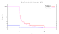 Escape time for C=0 and 0.5<Z<2.5
Math formula :

Maxima version :
GiveNormalizedIteration(z,c,E_R,i_Max):=
/* */
block(
 [i:0,r],
 while abs(z)<E_R and i<i_Max
   do (z:z*z + c,i:i+1),
 r:i-log2(log2(cabs(z))),
 return(float(r))
)$
In Maxima log(x) is a natural (base e) logarithm of x. To compute log2 use :
log2(x) := log(x) / log(2);
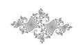
Level Curves of escape time Method = eLCM/J
 edge detection Image and C code
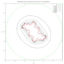 preimages of circle
These curves are boundaries of Level Sets of escape time ( eLSM/J ). They can be drawn using these methods:
- edge detection of Level Curves ( =boundaries of Level sets).
- Algorithm based on paper by M. Romera et al.[6]
- Sobel filter
- drawing lemniscates = curves , see explanation and source code
- drawing circle and its preimages. See this image, explanation and source code
- method described by Harold V. McIntosh[7]


/* Maxima code : draws lemniscates of Julia set */
c: 1*%i;
ER:2;
z:x+y*%i;
f[n](z) := if n=0 then z else (f[n-1](z)^2 + c);
load(implicit_plot); /* package by Andrej Vodopivec */
ip_grid:[100,100];
ip_grid_in:[15,15];
implicit_plot(makelist(abs(ev(f[n](z)))=ER,n,1,4),[x,-2.5,2.5],[y,-2.5,2.5]);
Basin of attraction of finite attractor = interior of filled-in Julia set
- How to find periodic attractor ?
- How many iterations is needed to reach attractor ?
Components of Interior of Filled Julia set ( Fatou set)
- use limited color ( palette = list of numbered colors)
- find period of attracting cycle
- find one point of attracting cycle
- compute number of iteration after when point reaches the attractor
- color of component=iteration % period[8]
- use edge detection for drawing Julia set
 Components of Fatou set for period 4
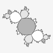 Components of Fatou set for period 3
 In case of Siegel disc critical orbit is a boundary Siegel disc compponent. All other componnats are preimages of this component
Internal Level Sets
See :
- algorithm 0 of program Mandel by Wolf Jung
 c = 0.5*i. Image and source code
 c = -0.584895. Image and source code
 Video for c along internal ray 0
Decomposition of target set
- Decomposition
 Binary decomposition of whole dynamical plane with circle Julia set c = 0
 Binary decomposition along internal ray 0
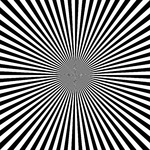 Modified binary decomposition of whole dynamical plane with circle Julia set. Image with src code
 Another modification of binary decomposition
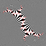 Modified decomposition of dynamical plane with dendrite Julia set. Image with src code
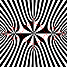 Modified decomposition of dynamical plane with basilica Julia set. Image with src code
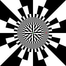
 from decomposition to parabolic checkerboard
Binary decomposition
Here color of pixel ( exterior of Julia set) is proportional to sign of imaginary part of last iteration .
Main loop is the same as in escape time.
In other words target set is decompositioned in 2 parts ( binary decomposition) :


Algorithm in pseudocode ( Im(Zn) = Zy ) :
if (LastIteration==IterationMax)
   then color=BLACK;   /* bounded orbits = Filled-in Julia set */
   else   /* unbounded orbits = exterior of Filled-in Julia set  */
        if (Zy>0) /* Zy=Im(Z) */
           then color=BLACK;
           else color=WHITE;
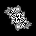
Modified decomposition
Here exterior of Julia set is decompositioned into radial level sets.
It is because main loop is without bailout test and number of iterations ( iteration max) is constant.
It creates radial level sets. See also video by bryceguy72[9] and by FreymanArt[10]
  for (Iteration=0;Iteration<8;Iteration++)
 /* modified loop without checking of abs(zn) and low iteration max */
    {
    Zy=2*Zx*Zy + Cy;
    Zx=Zx2-Zy2 +Cx;
    Zx2=Zx*Zx;
    Zy2=Zy*Zy;
   };
  iTemp=((iYmax-iY-1)*iXmax+iX)*3;
  /* --------------- compute  pixel color (24 bit = 3 bajts) */
 /* exterior of Filled-in Julia set  */
 /* binary decomposition  */
  if (Zy>0 )
   {
    array[iTemp]=255; /* Red*/
    array[iTemp+1]=255;  /* Green */
    array[iTemp+2]=255;/* Blue */
  }
  if (Zy<0 )
   {
    array[iTemp]=0; /* Red*/
    array[iTemp+1]=0;  /* Green */
    array[iTemp+2]=0;/* Blue */
  };
It is also related with automorphic function for the group of Mobius transformations [11]
Inverse Iteration Method (IIM/J) : Julia set
Inverse iteration of repellor for drawing Julia set
Complex potential - Boettcher coordinate
BSM/J
This algorithm is used when dynamical plane consist of two of more basins of attraction. For example for c=0.
It is not appropiate when interior of filled Julia set is empty, for example for c=i.
Description of algorithm :
- for every pixel of dynamical plane do :
- compute 4 corners ( vertices) of pixel ( where lt denotes left top, rb denotes right bottom, ... )
- check to which basin corner belongs ( standard escape time and bailout test )
- if corners do not belong to the same basin mark it as Julia set


Examples of code
DEM/J
This algorith has 2 versions :
- exterior
- interior
Compare it with version for parameter plane and Mandelbrot set : DEM/J
External distance estimation
 c=-0.74543+0.11301*i
 c= -0.75+0.11
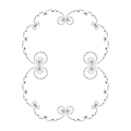 c = 0.255
 c=-0.1+0.651
" For distance estimate it has been proved that the computed value differs from the true distance at most by a factor of 4. " (Wolf Jung)
Math formula :

where :
is first derivative with respect to c.

This derivative can be found by iteration starting with

and then :

How to use distance
One can use distance for colouring :
- only Julia set ( boundary of filled Julia set)
- boundary and exterior of filled Julia set.
Here is first example :
if (LastIteration==IterationMax)
    then { /*  interior of Julia set, distance = 0 , color black */ }
    else /* exterior or boundary of Filled-in Julia set  */
         {  double distance=give_distance(Z0,C,IterationMax);
            if (distance<distanceMax)
                then { /*  Julia set : color = white */ }
                else  { /*  exterior of Julia set : color = black */}
         }
Here is second example [14]
if (LastIteration==IterationMax) or distance < distanceMax then ... // interior by ETM/J and boundary by DEM/J
else .... // exterior by real escape time
Zoom
DistanceMax is smaller than pixel size. During zooming pixel size is decreasing and DistanceMax should also be decreased to obtain good picture. It can be made by using formula :

where

One can start with n=1 and increase n if picture is not good. Check also iMax !!
DistanceMax may also be proportional to zoom factor [15] :


where thick is image width ( in world units) and mag is a zoom factor.
Examples of code
For cpp example see mndlbrot::dist from mndlbrot.cpp in src code of program mandel ver 5.3 by Wolf Jung.
C function :
/*based on function  mndlbrot::dist  from  mndlbrot.cpp
 from program mandel by Wolf Jung (GNU GPL )
 http://www.mndynamics.com/indexp.html  */
double jdist(double Zx, double Zy, double Cx, double Cy ,  int iter_max)
 {
 int i;
 double x = Zx, /* Z = x+y*i */
         y = Zy,
         /* Zp = xp+yp*1 = 1  */
         xp = 1,
         yp = 0,
         /* temporary */
         nz,
         nzp,
         /* a = abs(z) */
         a;
 for (i = 1; i <= iter_max; i++)
  { /* first derivative   zp = 2*z*zp  = xp + yp*i; */
    nz = 2*(x*xp - y*yp) ;
    yp = 2*(x*yp + y*xp);
    xp = nz;
    /* z = z*z + c = x+y*i */
    nz = x*x - y*y + Cx;
    y = 2*x*y + Cy;
    x = nz;
    /* */
    nz = x*x + y*y;
    nzp = xp*xp + yp*yp;
    if (nzp > 1e60 || nz > 1e60) break;
  }
 a=sqrt(nz);
 /* distance = 2 * |Zn| * log|Zn| / |dZn| */
 return 2* a*log(a)/sqrt(nzp);
 }
Delphi function :
function Give_eDistance(zx0,zy0,cx,cy,ER2:extended;iMax:integer):extended;

var zx,zy ,  // z=zx+zy*i
    dx,dy,  //d=dx+dy*i  derivative :  d(n+1)=  2 * zn * dn
    zx_temp,
    dx_temp,
    z2,  //
    d2, //
    a // abs(d2)
     :extended;
    i:integer;
begin
  //initial values
  // d0=1
  dx:=1;
  dy:=0;
  //
  zx:=zx0;
  zy:=zy0;
  // to remove warning : variables may be not initialised ?
  z2:=0;
  d2:=0;

  for i := 0 to iMax - 1 do
    begin
      // first derivative   d(n+1) = 2*zn*dn  = dx + dy*i;
      dx_temp := 2*(zx*dx - zy*dy) ;
      dy := 2*(zx*dy + zy*dx);
      dx := dx_temp;
      // z = z*z + c = zx+zy*i
      zx_temp := zx*zx - zy*zy + Cx;
      zy := 2*zx*zy + Cy;
      zx := zx_temp;
      //
      z2:=zx*zx+zy*zy;
      d2:=dx*dx+dy*dy;
      if ((z2>1e60) or (d2 > 1e60)) then  break;

    end; // for i
   if (d2 < 0.01) or (z2 < 0.1)  // when do not use escape time
    then  result := 10.0
    else
      begin
        a:=sqrt(z2);
        // distance = 2 * |Zn| * log|Zn| / |dZn|
        result := 2* a*log10(a)/sqrt(d2);
      end;

end;  //  function Give_eDistance
Matlab code by Jonas Lundgren[16]
function D = jdist(x0,y0,c,iter,D)
%JDIST Estimate distances to Julia set by potential function
% by Jonas Lundgren http://www.mathworks.ch/matlabcentral/fileexchange/27749-julia-sets
% Code covered by the BSD License http://www.mathworks.ch/matlabcentral/fileexchange/view_license?file_info_id=27749


% Escape radius^2
R2 = 100^2;

% Parameters
N = numel(x0);
M = numel(y0);
cx = real(c);
cy = imag(c);
iter = round(1000*iter);

% Create waitbar
h = waitbar(0,'Please wait...','name','Julia Distance Estimation');
t1 = 1;

% Loop over pixels
for k = 1:N/2
    x0k = x0(k);
    for j = 1:M
        % Update distance?
        if D(j,k) == 0
            % Start values
            n = 0;
            x = x0k;
            y = y0(j);
            b2 = 1;                 % |dz0/dz0|^2
            a2 = x*x + y*y;         % |z0|^2
            % Iterate zn = zm^2 + c, m = n-1
            while n < iter && a2 <= R2
                n = n + 1;
                yn = 2*x*y + cy;
                x = x*x - y*y + cx;
                y = yn;
                b2 = 4*a2*b2;       % |dzn/dz0|^2
                a2 = x*x + y*y;     % |zn|^2
            end
            % Distance estimate
            if n < iter
                % log(|zn|)*|zn|/|dzn/dz0|
                D(j,k) = 0.5*log(a2)*sqrt(a2/b2);
            end
        end
    end
    % Lap time
    t = toc;
    % Update waitbar
    if t >= t1
        str = sprintf('%0.0f%% done in %0.0f sec',200*k/N,t);
        waitbar(2*k/N,h,str)
        t1 = t1 + 1;
    end
end

% Close waitbar
close(h)
Maxima function :
GiveExtDistance(z0,c,e_r,i_max):=
/* needs z in exterior of Kc */
block(
[z:z0,
dz:1,
cabsz:cabs(z),
cabsdz:1, /* overflow limit */
i:0],
while  cabsdz < 10000000 and  i<i_max
 do
  (
   dz:2*z*dz,
   z:z*z + c,
   cabsdz:cabs(dz),
   i:i+1
  ),
 cabsz:cabs(z),
 return(2*cabsz*log(cabsz)/cabsdz)
)$
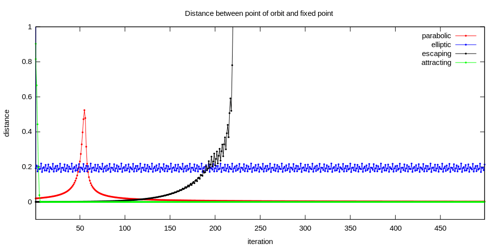
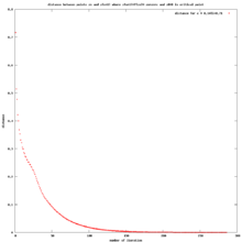
Convergence
In this algorithm distances between 2 points of the same orbit are checked
average discrete velocity of orbit
It is used in case of :
Cauchy Convergence Algorithm (CCA)
This algorithm is described by User:Georg-Johann. Here is also Matemathics code by Paul Nylander
Normality
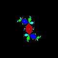
Normality In this algorithm distances between points of 2 orbits are checked
Checking equicontinuity by Michael Becker
"Iteration is equicontinuous on the Fatou set and not on the Julia set". (Wolf Jung) [17][18]
Michael Becker compares the distance of two close points under iteration on Riemann sphere.[19]
This method can be used to draw not only Julia sets for polynomials ( where infinity is always superattracting fixed point) but it can be also applied to other functions ( maps), for which infinity is not an attracting fixed point.[20]
using Marty's criterion by Wolf Jung
Wolf Jung is using "an alternative method of checking normality, which is based on Marty's criterion: |f'| / (1 + |f|^2) must be bounded for all iterates." It is implemented in mndlbrot::marty function ( see src code of program Mandel ver 5.3 ). It uses one point of dynamic plane.
Koenigs coordinate
Koenigs coordinate are used in the basin of attraction of finite attracting (not superattracting) point (cycle).
Optimisation
Distance
You don't need a square root to compare distances. [21]
Symmetry
Julia sets can have many symmetries [22][23]
Quadratic Julia set has allways rotational symmetry ( 180 degrees) :
colour(x,y) = colour(-x,-y)
when c is on real axis ( cy = 0) Julia set is also reflection symmetric :[24]
colour(x,y) = colour(x,-y)
Algorithm :
- compute half image
- rotate and add the other half
- write image to file [25]
Color
- color in computer graphic
- Visualising Julia sets by Georg-Johann
- Combined Methods of Depicting Julia Sets and Parameter Planes by Chris King
- On Fractal Coloring Techniques by Jussi Harkonen Master's Thesis, Department of Mathematics, Åbo Akademi University, Turku, 2007, 61 pages. The thesis was carried out under the supervision of Professor Goran Hognas
- Technical Info - Colorizing by Michael Condron
Sets
Target set
Target set or trap
One can divide it according to :
- attractors ( finite or infinite)
- dynamics ( hyperbolic, parabolic, elliptic )
For infinite attractor - hyperbolic case
Target set is an arbitrary set on dynamical plane containing infinity and not containing points of Filled-in Fatou sets.

For escape time algorithms target set determines the shape of level sets and curves. It does not do it for other methods.
Exterior of circle
This is typical target set. It is exterior of circle with center at origin and radius =ER :


Radius is named escape radius ( ER ) or bailout value. Radius should be greater than 2.
Exterior of square
Here target set is exterior of square of side length centered at origin


For finite attractors
See :
- Internal Level Sets
- Binary decomposition
- Tessellation of the Interior of Filled Julia Sets by Tomoki KAWAHIRA [26]
Julia sets
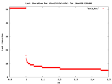
"Most programs for computing Julia sets work well when the underlying dynamics is hyperbolic but experience an exponential slowdown in the parabolic case." ( Mark Braverman )[27]
- when Julia set is a set of points that do not escape to infinity under iteration of the quadratic map ( = filled Julia set has no interior = dendrt)
- IIM/J
- DEM/J
- checking normality
- when Julia set is a boundary between 2 basin of attraction ( = filled Julia set has no empty interior) :
- boundary scaning [28]
- edge detection
Fatou set
Interior of filled Julia set can be coloured :
- speed of attraction ( integer value = the number of iterations used to guess if a point is in the set ) which is coverted to colour ( or shade of gray ) [29]
- Internal Level Sets
- attracting time ( sth like escape time but checks if (abs(z-attractor)<Attracting_radius
- Binary decomposition
- Tessellation of the Interior of Filled Julia Sets by Tomoki KAWAHIRA [30]
- discrete veolocity in Siegel disc case
Periodic points
More is here
Video
One can make videos using :
- zoom into dynamic plane
- changing parametr c along path inside parameter plane[31]
- changing coloring scheme ( for example color cycling )
Examples :
- Target set for internal ray 0 video
- Quadratic Julia set with Internal level sets for internal ray 0 video
More tutorials and code
- in Java see Evgeny Demidov
- in C see :
- in C++ see Wolf Jung page,
- in Gnuplot see Tutorial by T.Kawano
- in Lisp for Maxima see Dynamics by Jaime E. Villate
- in Mathemathica see :
References
- ↑ Standard coloring algorithms from Ultra Fractal
- ↑ Faster Fractals Through Algebra by Bruce Dawson ( author of Fractal eXtreme)
- ↑ C code with gsl from tensorpudding
- ↑ Program Mandel by Wolf Jung on GNU General Public License
- ↑ Euler examples by R. Grothmann
- ↑ Drawing the Mandelbrot set by the method of escape lines. M. Romera et al.
- ↑ Julia Curves, Mandelbrot Set, Harold V. McIntosh.
- ↑ The fixed points and periodic orbits by E Demidov
- ↑ Video : Julia Set Morphing with Magnetic Field lines by bryceguy72
- ↑ Video : Mophing Julia set with color bands / stripes by FreymanArt
- ↑ Gerard Westendorp : Platonic tilings of Riemann surfaces - 8 times iterated Automorphic function z->z^2 -0.1+ 0.75i
- ↑ Pascal program fo BSM/J by Morris W. Firebaugh
- ↑ Boundary scanning and complex dynamics by Mark McClure
- ↑ Pictures of Julia and Mandelbrot sets by Gert Buschmann
- ↑ Pictures of Julia and Mandelbrot sets by Gert Buschmann
- ↑ Julia sets by Jonas Lundgren in Matlab
- ↑ Alan F. Beardon, S. Axler, F.W. Gehring, K.A. Ribet : Iteration of Rational Functions: Complex Analytic Dynamical Systems. Springer, 2000; ISBN 0387951512, 9780387951515; page 49
- ↑ Joseph H. Silverman : The arithmetic of dynamical systems. Springer, 2007. ISBN 0387699031, 9780387699035; page 22
- ↑ Visualising Julia sets by Georg-Johann
- ↑ Julia sets by Michael Becker. See the metric d(z,w)
- ↑ Algorithms : Distance_approximations in wikibooks
- ↑ The Julia sets symmetry by Evgeny Demidov
- ↑ mathoverflow : symmetries-of-the-julia-sets-for-z2c
- ↑ htJulia Jewels: An Exploration of Julia Sets by Michael McGoodwin (March 2000)
- ↑ julia sets in Matlab by Jonas Lundgren
- ↑ Tessellation of the Interior of Filled Julia Sets by Tomoki Kawahira
- ↑ Mark Braverman : On efficient computation of parabolic Julia sets
- ↑ ALGORITHM OF COMPUTER MODELLING OF JULIA SET IN CASE OF PARABOLIC FIXED POINT N.B.Ampilova, E.Petrenko
- ↑ Ray Tracing Quaternion Julia Sets on the GPU by Keenan Crane
- ↑ Tessellation of the Interior of Filled Julia Sets by Tomoki Kawahira
- ↑ Julia-Set-Animations at devianart
- Drakopoulos V., Comparing rendering methods for Julia sets, Journal of WSCG 10 (2002), 155–161
- tree with dynamics by Nathaniel D. Emerson
- "Spiral Structures in Julia Sets and Related Sets", M. Michelitsch and O. E. Roessler in a book : SPIRAL SYMMETRY I. Hargittai and C. Pickover. (1992) World Scientific Publishing,
- The Evolution of a Three-armed Spiral in the Julia Set, and Higher Order Spirals", A. G. Davis Philip in a book : SPIRAL SYMMETRY I. Hargittai and C. Pickover. (1992) World Scientific Publishing,
- Beardon, A. : Symmetries of julia sets. The Mathematical Intelligencer. 1996-03-01 Springer New York Issn: 0343-6993 page 43 - 44.