Engineering Analysis/Matrices

Derivatives

Consider the following set of linear equations:

a = bx_1 + cx_2

d = ex_1 + fx_2

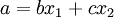
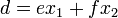
We can define the matrix A to represent the coefficients, the vector B as the results, and the vector x as the variables:

A = \begin{bmatrix}b & c \\ e & f\end{bmatrix}

B = \begin{bmatrix}a \\ d\end{bmatrix}

x = \begin{bmatrix}x_1 \\ x_2\end{bmatrix}

And rewriting the equation in terms of the matrices, we get:

B = Ax

Now, let's say we want the derivative of this equation with respect to the vector x:

\frac{d}{dx}B = \frac{d}{dx}Ax

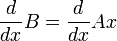
We know that the first term is constant, so the derivative of the left-hand side of the equation is zero. Analyzing the right side shows us:

Pseudo-Inverses

There are special matrices known as pseudo-inverses, that satisfies some of the properties of an inverse, but not others. To recap, If we have two square matrices A and B, that are both n × n, then if the following equation is true, we say that A is the inverse of B, and B is the inverse of A:

AB = BA = I

Right Pseudo-Inverse

Consider the following matrix:

R = A^T[AA^T]^{-1}

We call this matrix R the right pseudo-inverse of A, because:

AR = I

but

RA \ne I

We will denote the right pseudo-inverse of A as $A^\dagger$

Left Pseudo-Inverse

Consider the following matrix:

L = [A^TA]^{-1}A^T

We call L the left pseudo-inverse of A because

LA = I

but

AL \ne I

We will denote the left pseudo-inverse of A as $A^\ddagger$

This article is issued from Wikibooks. The text is licensed under Creative Commons - Attribution - Sharealike. Additional terms may apply for the media files.