Circuit Theory/TF Objectives

< Circuit Theory

Thevenin/Norton impedance completely characterizes a circuit from a load's point of view. Differential equations completely describe a circuit. The impulse response of a circuit is all that is needed to use the convolution integral. Phasors and complex frequencies completely describe a circuit. And even while computing the transient response, complex frequencies associated with the steady state sinusoidal response appeared. Are they all related? Yes.

The goal is to understand all the above as a transfer function. Why? Most engineering uses this concept. Here are some electrical applications:

Analog Computers ... (modeling before digital computers)
Signal Processing ... (wireless, cable communication)
Control theory ... (motors don't die and don't spin out of control when the load changes)
Linear time-invariant system theory ... (general math model which assumes the values of resistors, inductors and capacitors don't vary over time, temperature, bias .. but provides a good starting point for establishing expectations and experimenting)

The goal is to introduce transfer functions in the context of electronics.

Transfer Function Definition

A Transfer Function is the ratio of the output of a system to the input of a system. If we have an input function of X(s), and an output function Y(s), we define the transfer function H(s) to be:

H(s) = {Y(s) \over X(s)}

Four RLC Transfer Functions

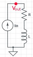
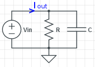
In the context of RLC circuits, transfer functions are in a phasor/complex frequency/laplace domain concept. They are not a time domain concept. They are independent of the forcing function/source. There are four possible RLC transfer patterns:

$\frac{output}{input}$	Example Circuit	Transfer Function
${\frac {V_{out}(s)}{I_{in}(s)}}$	impedance	$H(s)=R+Ls$
${\frac {I_{out}(s)}{V_{in}(s)}}$	admittance	$H(s)={\frac {1}{R}}+Cs$
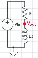${\frac {V_{out}(s)}{V_{in}(s)}}$	voltage divider	$H(s)={\frac {Ls}{R+Ls}}$
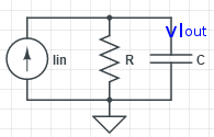${\frac {I_{out}(s)}{I_{in}(s)}}$	current divider	$H(s)={\frac {Cs}{{\frac {1}{R}}+Cs}}$

Applications

The transfer function has many applications as we will soon see. But it's immediate benefit is eliminating the need to find the differential equation. Reviewing previous examples:

Example	Differential Equation	Transfer Function
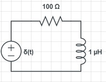
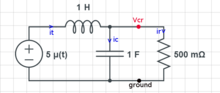
convolution integral problem Given voltage source, find total current	: $v(t)=L{di(t) \over dt}+Ri(t)$	admittance: $H(s)={\frac {\mathbb {I} (s)}{\mathbb {V} (s)}}={\frac {1}{sL+R}}$
Second Order, Source Excitement Find i_o giving Is	$I_{s}={d^{2}i_{o} \over dt^{2}}+2{di_{o} \over dt}+2i_{o}$	current divider: $H(s)={\frac {\mathbb {I} _{o}(s)}{\mathbb {I} _{s}(s)}}={\frac {\frac {1}{R+Ls}}{{\frac {1}{R+Ls}}+{\frac {1}{R}}+Cs}}$ $H(s)={\frac {\mathbb {I} _{o}(s)}{\mathbb {I} _{s}(s)}}={\frac {1}{s^{2}+2s+2}}$ R :=1; L :=1; C :=1; simplify((1/(R + Ls))/(1/(R + Ls) + 1/R + C*s))
Second Order, Source Excitement Given V_s, find V_cr	$V_{s}(t)=L{d({\frac {V_{CR}}{R}}) \over dt}+LC{d^{2}(V_{CR} \over dt^{2}})+V_{CR}$	Voltage Divider $H(s)={\frac {\mathbb {V} _{cr}(s)}{\mathbb {V} _{s}(s)}}={\frac {\frac {1}{{\frac {1}{R}}+Cs}}{{\frac {1}{{\frac {1}{R}}+Cs}}+Ls}}$ $H(s)={\frac {1}{CLs^{2}+{\frac {Ls}{R}}+1}}$

Interpreting Complex Roots

After finding the transfer function, the next step is finding the time constant or the complex frequency roots and from these guess the form of the solution.

The homogeneous solution is found by setting the denominator of the transfer function to zero. Factoring the denominator and finding the complex frequency roots is called finding "zeros."

The numerator (which was one in all the above examples) may have a complex frequency polynomial (in complicated circuits) that can also be set equal to zero. The roots are called "poles." Poles influence the circuit's response to different frequencies rather than the time domain response.

Summarizing Time

This ends the normal circuit theory course. Time domain analysis could continue and this is hinted at in the following example. Before WWII it was important to continue in order to model physical systems with analog computers. But today, digital computers can model much more accurately. So stopping time analysis here leaves further study for a specialized class. Let's summarize what we have learned about circuits in the time domain.

Superposition allows replacing multiple sources with one source at a time (zeroing the others) and then adding the results of all sources.
Impedance, admittance, voltage divider and current divider formulas lead directly to the differential equations ... which is the same math for phasor/complex frequency and the Laplace domain.
The Convolution integral eliminates the need to transform driving functions (particularly sinusoidal) into the phasor/complex frequency/Laplace domain. Instead the source is replaced with 1 volt or 1 amp, and the particular solution turns into a DC final condition (t = ∞) placed on the homogeneous solution and appears with in the differential equation constant.

This article is issued from Wikibooks. The text is licensed under Creative Commons - Attribution - Sharealike. Additional terms may apply for the media files.